Penalised regression improves imputation of cell-type specific expression using RNA-seq data from mixed cell populations compared to domain-specific methods

Modified

23-Jan-25

[1] "/rds/project/rds-csoP2nj6Y6Y/wyl37/Rbookdown/sceQTLGen/CLUSTERdeconRes"

1 Main Figures

1.1 Figure1, multi-response LASSO/ridge

multi-response LASSO/ridge to predict sample-level cell-type expression

1.2 Figure 2, Data and study design

CLUSTER samples by cell type (row) and subject (column). Cells are coloured based on the availability of RNA (Y for yes, N for no), and the top panel annotations indicate the RNA sequencing batch (Batch).

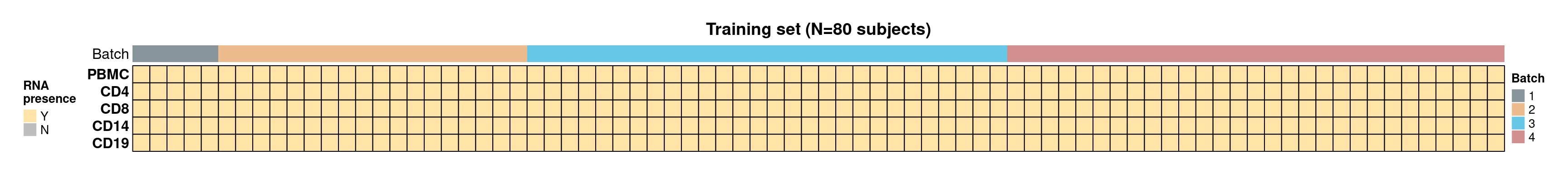
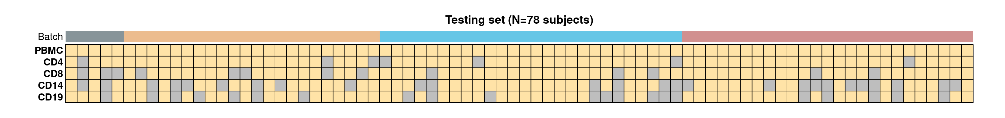
Data analysis workflow. Transcripts per million (TPM) were calculated after excluding low-expressed genes. TPM from sorted cells (CD4, CD8, CD14, and CD19) from 80 training samples were used to generate custom signature genes using the CIBERSORTxFractions module. We deconvoluted the cell fractions from PBMC based on inbuilt and custom signatures using CIBERSORTx, using the custom signature genes with bMIND and cell-type specific genes using debCAM. Estimates of cell fractions were compared to the ground-truth cell fractions from flow cytometry, and we assessed fraction accuracy using Pearson correlation and RMSE (root mean square error). Next, we estimated sample-level cell-type gene expression based on inbuilt and custom signature matrices using the CIBERSORTx high resolution module. In parallel, we ran bMIND and swCAM, with the flow cytometry cell fractions, in a supervised mode for estimating cell-type expression. For each cell type, we trained a LASSO/RIDGE model on PBMC and sorted cells with 5-fold cross-validation and used this to predict cell-type gene expression in the test samples. We compared imputed cell-type expressions with the observed ones and evaluated and benchmarked the performance using Pearson correlation, RMSE and a novel measure, differential gene expression (DGE) recovery.

1.3 Figure 3, Prediction accuracy of cell fractions

Code

####################
## flow fractions ##
####################
fractflow <- file.path(
  data_dir,
  "CLUSTERData/flowFract_wide.rds"
) %>%
  readRDS()



## cibx-LM22
#############################
## fractions based on LM22 ##
#############################
lm22merged <- "data4repo/mergedClasses.csv" %>%
  file.path(here::here(), .) %>%
  scan(., what = "character", sep = "\t")

res_d <- file.path("CIBXres/LM22deconv", runid) %>%
  file.path(data_dir, .)
res_d
[1] "/rds/project/rds-csoP2nj6Y6Y/wyl37/Rbookdown/sceQTLGen/CLUSTERdeconRes/CIBXres/LM22deconv/cluster"

lm22mtx <- file.path(res_d, "sigMTX4dev.txt") %>%
  fread()

lm22res <- file.path(res_d, "CIBERSORTxGEP_NA_Fractions-Adjusted.txt") %>%
  fread()

stopifnot(names(lm22res)[-1][1:length(names(lm22mtx)[-1])] == names(lm22mtx)[-1])

## fractions in 22 cell types
lm22res.mtx <- lm22res[, names(lm22mtx)[-1], with = FALSE] %>% as.matrix()
rownames(lm22res.mtx) <- lm22res$Mixture

## fractions merged into 4 cell types based on lm22merged
lm22res.4ct <- matrix(NA, nrow = nrow(lm22res.mtx), ncol = length(sctorder))
rownames(lm22res.4ct) <- lm22res$Mixture

for (n in seq_along(sctorder)) {
  colidx <- which(lm22merged == sctorder[n])
  lm22res.4ct[, n] <- rowSums(lm22res.mtx[, colidx, drop = FALSE])
}

## merged class for 4 sorted cells
ctlm22pooled <- lapply(sctorder, function(ct) {
  colnames(lm22res.mtx)[lm22merged == ct]
})
names(ctlm22pooled) <- sctorder

## fractions of 4 cell types scaled to 1
lm22res.4ct.scaled <- apply(lm22res.4ct, 1, function(x) 1 / sum(x) * x) %>% t()
colnames(lm22res.4ct.scaled) <- sctorder
lm22res.4ct.scaled <- lm22res.4ct.scaled[rownames(fractflow), ]

##################
## sorted cells ##
##################
res_d <- file.path("CIBXres/deconv", runid) %>%
  file.path(data_dir, .)
res_d
[1] "/rds/project/rds-csoP2nj6Y6Y/wyl37/Rbookdown/sceQTLGen/CLUSTERdeconRes/CIBXres/deconv/cluster"

customfract <- file.path(res_d, "CIBERSORTxGEP_NA_Fractions.txt") %>%
  fread()
customres <- customfract[, ..sctorder] %>% as.matrix()
rownames(customres) <- customfract$Mixture
customres <- customres[rownames(fractflow), ]

###########
## bMIND ##
###########
res_d <- file.path("bMINDres", runid) %>%
  file.path(data_dir, .)
res_d
[1] "/rds/project/rds-csoP2nj6Y6Y/wyl37/Rbookdown/sceQTLGen/CLUSTERdeconRes/bMINDres/cluster"

bmindresFract <- readRDS(file.path(res_d, "bMIND_Fractres.rds"))[["frac"]]
bmindresFract <- bmindresFract[rownames(fractflow), ]

############
## debCAM ##
############
res_d <- file.path("swCAMres", runid) %>%
  file.path(data_dir, .)
res_d
[1] "/rds/project/rds-csoP2nj6Y6Y/wyl37/Rbookdown/sceQTLGen/CLUSTERdeconRes/swCAMres/cluster"

## 4 fold changes (FC) for marker selection
debCAMresFract <- readRDS(file.path(res_d, "debCAM_FractresPure80.rds"))
debCAMresFract %>% names() # OVER.FC_1, FC_2, FC_5, FC_10
[1] "OVE.FC_1"  "OVE.FC_2"  "OVE.FC_5"  "OVE.FC_10"

## go for fraction results based on FC10
debFract <- debCAMresFract$OVE.FC_10$Aest[rownames(fractflow), ]

#######################
## flow + pred fract ##
#######################
## true fraction longformat
flowfract.m <- copy(fractflow) %>%
  setDT(., keep.rownames = TRUE) %>%
  melt(
    data = .,
    id.vars = c("rn"),
    measure.vars = sctorder,
    variable.name = "celltype",
    variable.factor = FALSE,
    value.name = "flowfract"
  ) %>%
  setnames(., "rn", "sampleName")

## pred fraction in

fract_appro <- c("CIBX-inbuilt", "CIBX-custom", "bMIND-custom", "debCAM")

predfract <- list(
  lm22res.4ct.scaled,
  customres,
  bmindresFract,
  debFract
)
names(predfract) <- fract_appro

pltfract <- lapply(names(predfract), function(dat) {
  dsn <- as.data.frame(predfract[[dat]]) %>% setDT(., keep.rownames = TRUE)
  dsn.m <- melt(
    data = dsn,
    id.vars = c("rn"),
    measure.vars = sctorder,
    variable.name = "celltype",
    variable.factor = FALSE,
    value.name = "predfract",
  )
  dsn.m[, frt_type := dat]
  setnames(dsn.m, "rn", "sampleName")

  dsn.m[flowfract.m, flowfract := i.flowfract, on = c("sampleName", "celltype")]

  dsn.m
}) %>% rbindlist(., use.names = TRUE)

## limited to test samples
pltfract_test <- pltfract[sampleName %in% sampdata[samtype != "refsamp", sample], ]
pltfract_test[, ":="(
  frt_type = factor(frt_type, levels = fract_appro),
  celltype = factor(celltype, levels = sctorder)

)]

## r & rmse
cordsn <- pltfract_test[,
  {
    rhores <- cor(flowfract, predfract)
    rmse <- sqrt(mean((flowfract - predfract)^2))
    list(rhores, rmse)
  },
  by = c("frt_type", "celltype")
][, tlab := paste0("R=", round(rhores, 2), "\n", "RMSE=", round(rmse, 3))]

fig2plt <- ggpubr::ggscatter(
  data = pltfract_test,
  x = "flowfract", y = "predfract",
  fill = "celltype", shape = 21, size = 2,
  facet.by = c("frt_type", "celltype"),
  alpha = 1,
  palette = ctfrat.pal,
  position = "jitter",
  xlab = "Flow Fraction",
  ylab = "Predicted Fraction"
) +
  geom_abline(slope = 1, intercept = 0, linetype = 2, color = "blue") +
  facet_grid(frt_type ~ celltype, scales = "fixed") +
  ggpp::geom_text_npc(
    aes(
      npcx = 0.05, npcy = 0.97,
      label = tlab
    ),
    size = 3.5,
    data = cordsn
  ) +
  used_ggthemes(
    strip.text.y.right = element_text(angle = 0),
    legend.position = "none"
  )

Prediction accuracy of cell fractions by cell type (column) and approaches (row). Pearson correlation (R) and root mean square errors (RMSE) were calculated between estimated fractions (y-axis) and flow cytometry measures (x-axis). Each point is a testing sample and dashed blue lines indicate \(y = x\). CIBX-inbuilt: CIBERSORTx fraction deconvolution using the inbuilt signature matrix; CIBX-custom: CIBERSORTx fraction deconvolution using the custom signature matrix; bMIND-custom: bMIND fraction estimation using the custom signature matrix; debCAM-custom: debCAM fraction estimation using cell-type specific genes.

Code

fig2plt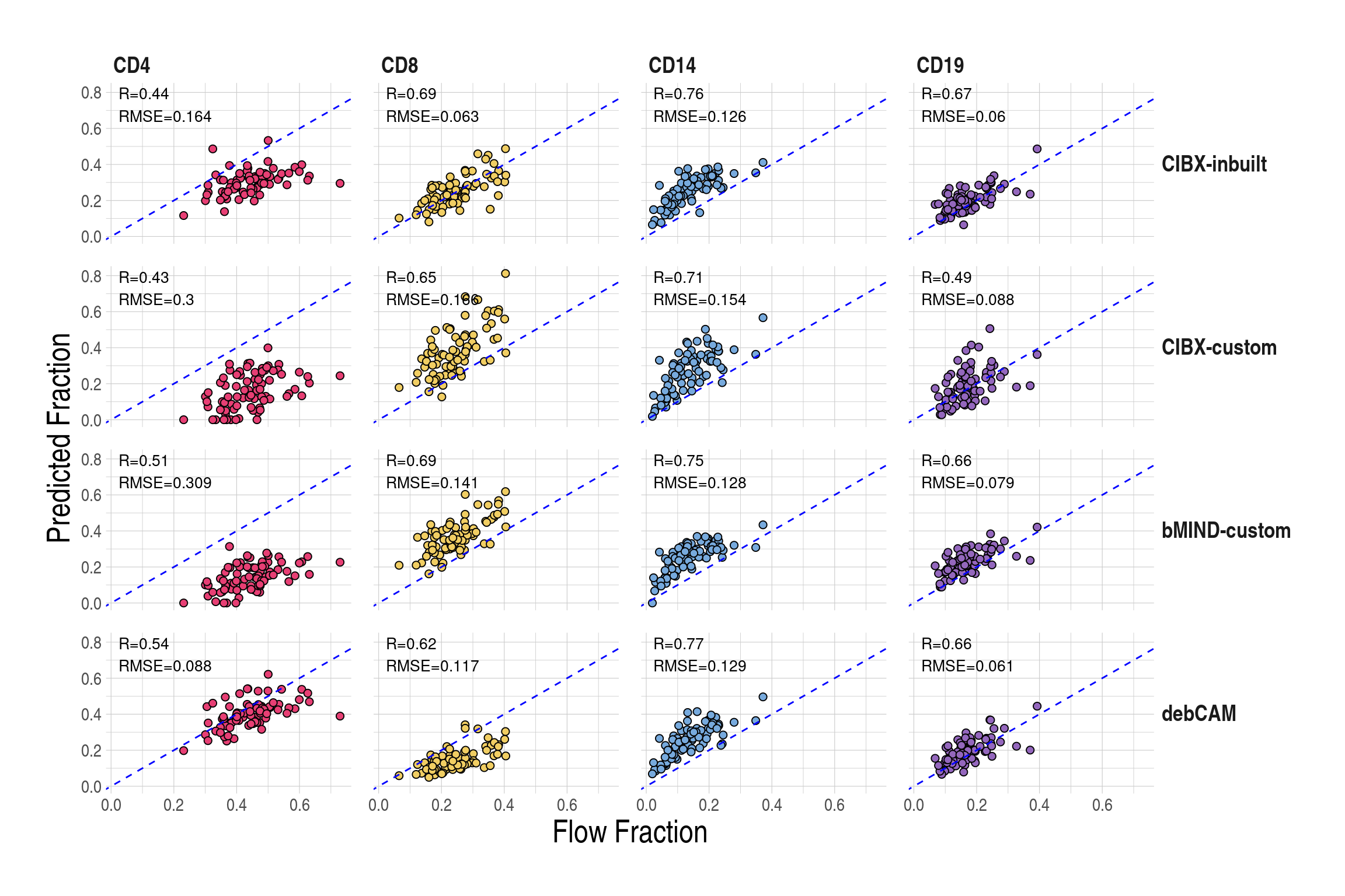

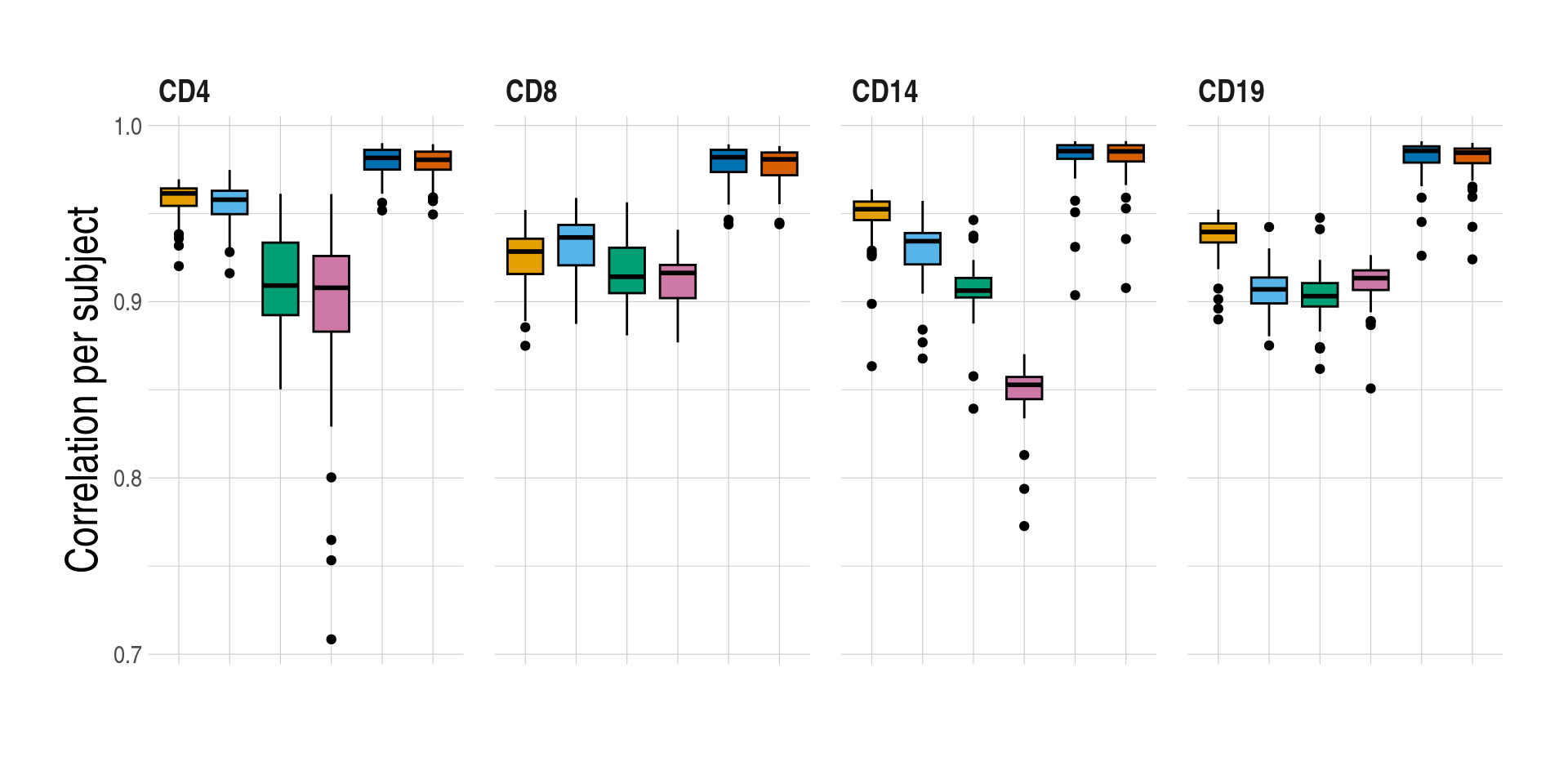
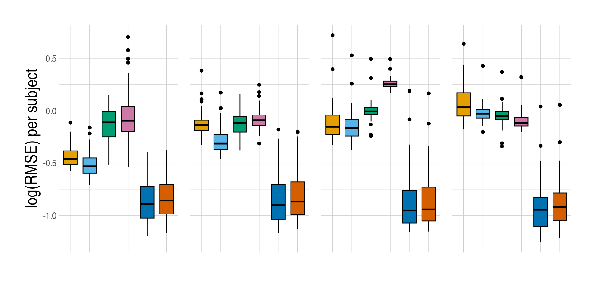
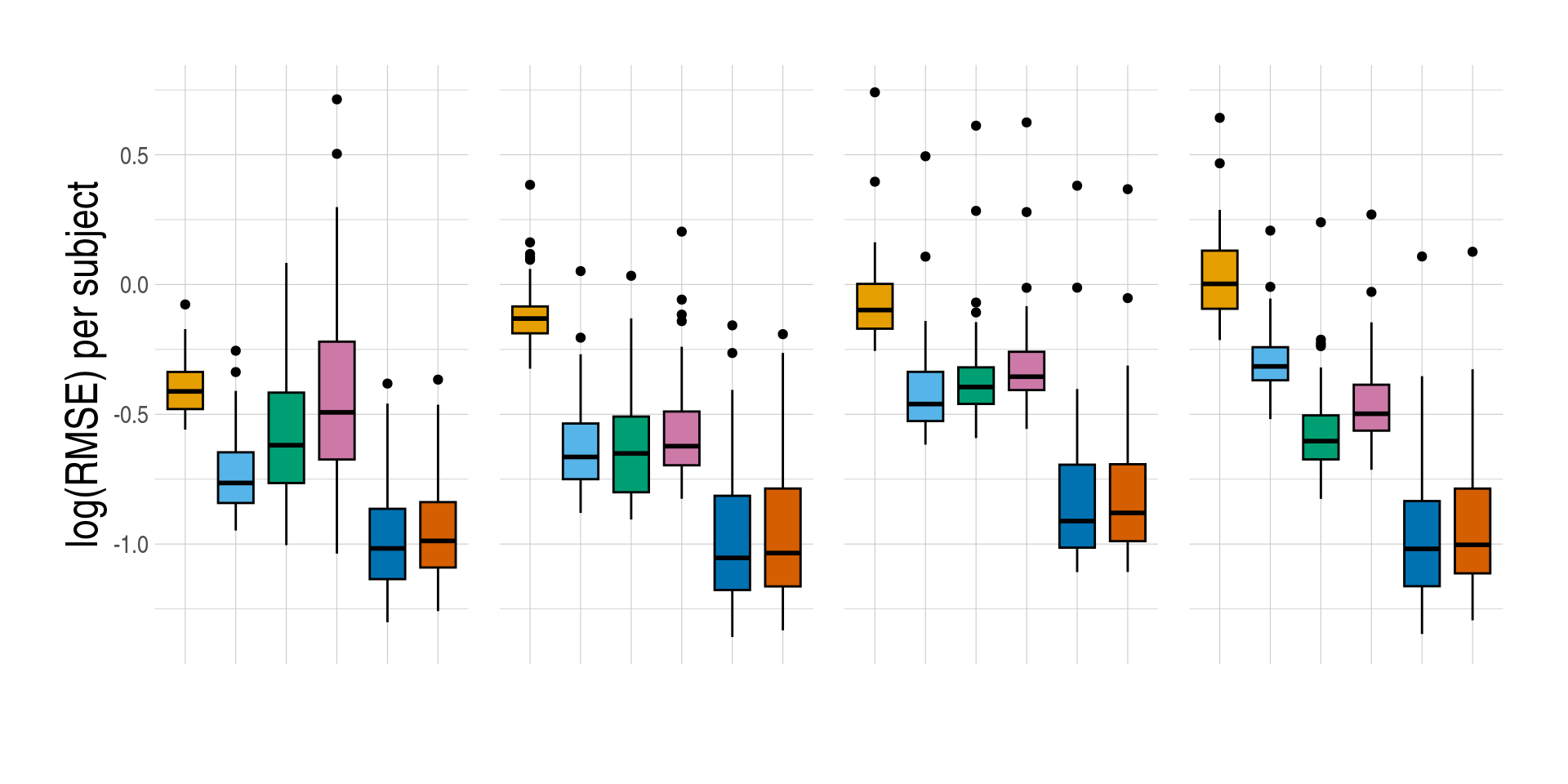
1.4 Figure 4, Prediction accuracy of cell-type expression

Distributions of prediction accuracy by cell type and approach. Prediction accuracy was evaluated by calculating Pearson correlation and root mean square error (RMSE) between observed and predicted cell-type expression across genes for the same subjects by cell type and approach. The approaches used were: inbuilt - CIBERSORTx expression deconvolution with the inbuilt signature matrix, custom - CIBERSORTx expression deconvolution with a custom signature matrix derived from sorted cell-type expression in training samples, bMIND - bMIND expression deconvolution with flow fractions, swCAM - swCAM deconvolution with flow fractions, and LASSO/RIDGE - expression predicted from regularised multi-response Gaussian models.

Code

## expression from approaches
cdata_explst <- prep_dat(
  rid = "cluster",
  res_dir = data_dir,
  cluster = TRUE
)

## predicted accuracy

numCores <- length(expr_order)
cl <- makeCluster(numCores, type = "FORK")
registerDoParallel(cl)

pedaccdsn_persub <- foreach(i = expr_order, .combine = "rbind") %dopar% {
  run_fig3v(
    obvexpr = cdata_explst$oexpr, impvexpr = cdata_explst$iexpr,
    sce = i, ct = sctorder, persub = TRUE
  ) %>%
    rbindlist()
}

stopCluster(cl)


pedaccdsn_persub[, .N, by = c("approach", "celltype")]

pedaccdsn_persub[, ":="(
  approach = factor(approach, levels = expr_order),
  celltype = factor(celltype, levels = sctorder)
)][, measure_rmse := log(measure_rmse)]


measureii <- c("Correlation per subject", "log(RMSE) per subject")
names(measureii) <- c("measure_cor", "measure_rmse")

lapply(seq_along(measureii), function(idx) {
  bplt <- ggboxplot(
    data = pedaccdsn_persub,
    x = "approach",
    xlab = "",
    y = names(measureii)[idx],
    ylab = measureii[idx],
    fill = "approach",
    palette = appro.cols %>% as.vector(),
    facet.by = c("celltype")
  ) +
    facet_grid(~celltype, scales = "free")

  if (idx == 1) {
    bplt <- bplt +
      used_ggthemes(
        axis.text.x = element_blank(),
        legend.position = "none"
      )
  } else {
    bplt <- bplt +
      used_ggthemes(
        axis.text.x = element_blank(),
        legend.position = "none",
        strip.text = element_blank()
      )
  }

  bplt
})

Code

numCores <- length(expr_order)
cl <- makeCluster(numCores, type = "FORK")
registerDoParallel(cl)

pedaccdsn <- foreach(i = expr_order, .combine = "rbind") %dopar% {
  run_fig3v(
    obvexpr = cdata_explst$oexpr, impvexpr = cdata_explst$iexpr,
    sce = i, ct = sctorder, persub = FALSE
  ) %>%
    rbindlist()
}

stopCluster(cl)


pedaccdsn[, .N, by = c("approach", "celltype")]
    approach celltype     N
 1:  inbuilt      CD4  6261
 2:  inbuilt      CD8  8003
 3:  inbuilt     CD14  7522
 4:  inbuilt     CD19  5779
 5:   custom      CD4  7241
 6:   custom      CD8 11794
 7:   custom     CD14  7823
 8:   custom     CD19  5881
 9:    bMIND      CD4 18871
10:    bMIND      CD8 18871
11:    bMIND     CD14 18821
12:    bMIND     CD19 18864
13:    swCAM      CD4 18871
14:    swCAM      CD8 18870
15:    swCAM     CD14 18867
16:    swCAM     CD19 18871
17:    LASSO      CD4 18871
18:    LASSO      CD8 18871
19:    LASSO     CD14 18053
20:    LASSO     CD19 18854
21:    RIDGE      CD4 18871
22:    RIDGE      CD8 18871
23:    RIDGE     CD14 18555
24:    RIDGE     CD19 18747
    approach celltype     N

pedaccdsn[, ":="(
  approach = factor(approach, levels = expr_order),
  celltype = factor(celltype, levels = sctorder)
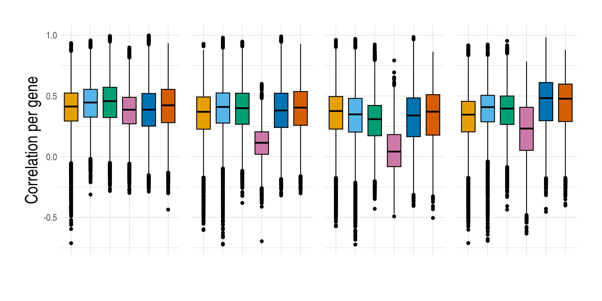
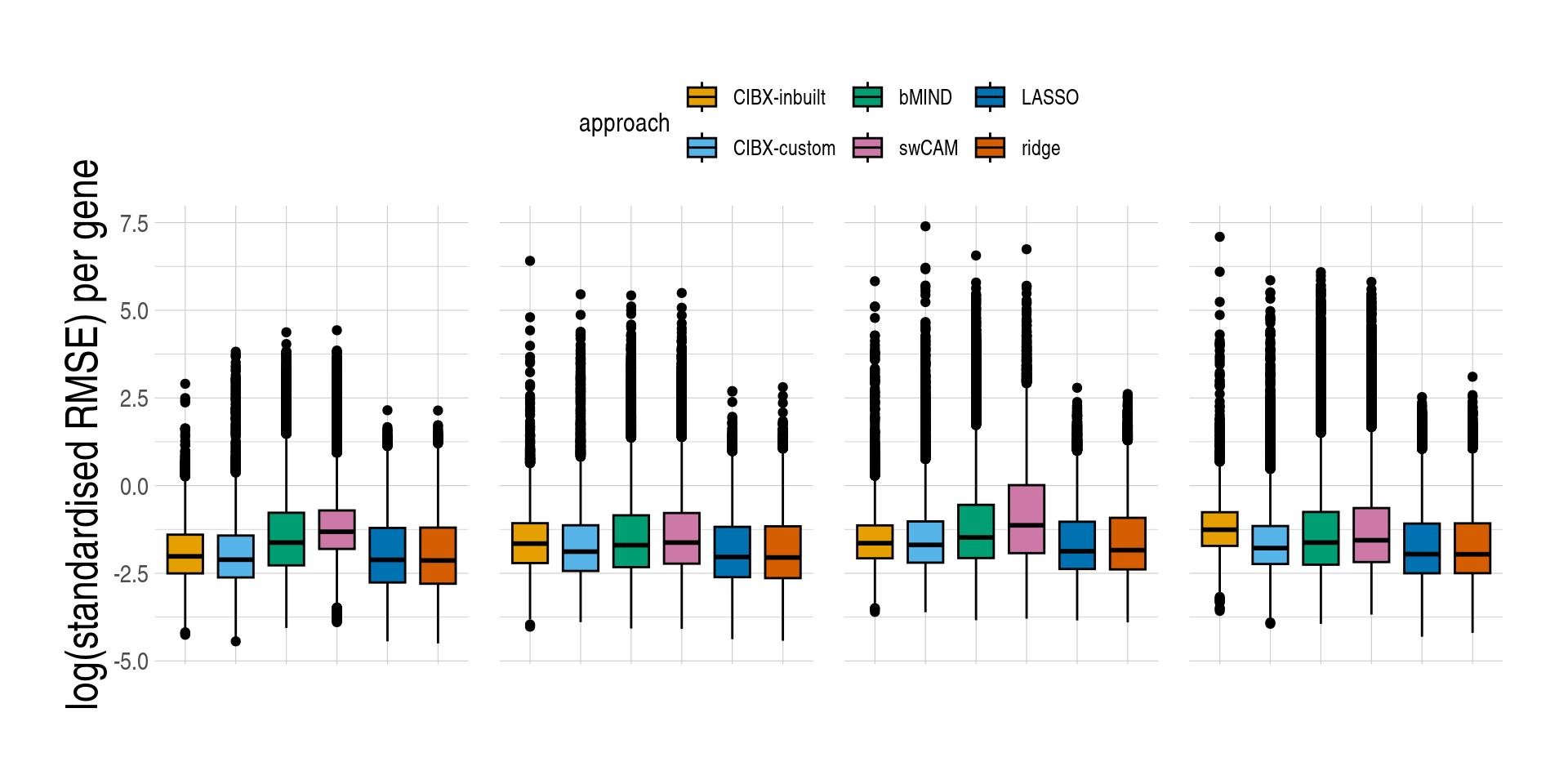
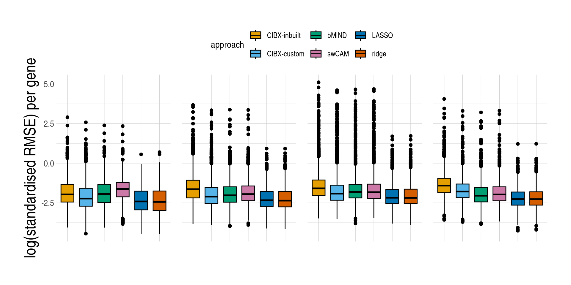
)][, measure_rmse := log(measure_rmse)]

Distributions of prediction accuracy by cell type and approach. Prediction accuracy was evaluated by calculating Pearson correlation and root mean square error (RMSE) between observed and predicted cell-type expression across testing samples for each gene by cell type and approach. Standardised RMSEs: RMSE/average observed expression. The approaches used were: inbuilt - CIBERSORTx expression deconvolution with the inbuilt signature matrix, custom - CIBERSORTx expression deconvolution with a custom signature matrix derived from sorted cell-type expression in training samples, bMIND - bMIND expression deconvolution with flow fractions, swCAM - swCAM deconvolution with flow fractions, and LASSO/RIDGE - expression predicted from regularised multi-response Gaussian models.

Code

measureii <- c("Correlation per gene", "log(standardised RMSE) per gene")
names(measureii) <- c("measure_cor", "measure_rmse")

lapply(seq_along(measureii), function(idx) {
  aplt <- ggboxplot(
    data = pedaccdsn,
    x = "approach",
    xlab = "",
    y = names(measureii)[idx],
    ylab = measureii[idx],
    fill = "approach",
    palette = appro.cols %>% as.vector(),
    facet.by = c("celltype")
  ) +
    scale_fill_manual(labels = appro_lab, values = appro.cols) +
    facet_grid(~celltype, scales = "free")

  if (idx == 1) {
    aplt <- aplt +
      used_ggthemes(
        axis.text.x = element_blank(),
        legend.position = "none",
        strip.text = element_blank()
      )
  } else {
    aplt <- aplt +
      used_ggthemes(
        axis.text.x = element_blank(),
        legend.position = "top",
        strip.text = element_blank()
      )
  }


  aplt
})

Code

fig4_f <- "fig4res.rds"

if (!file.exists(fig4_f)) {
  ## prepare data to run fig4
  myrunfig4 <- run_datprepfig4(
    obvexpr = cdata_explst$oexpr,
    impvexpr = cdata_explst$iexpr,
    tsampct = cdata_explst$trainsamp
  )

  names(myrunfig4)

  ## dge & roc
  fig4res <- run_fig4(myrunfig4)

  names(fig4res)

  saveRDS(fig4res, file = fig4_f)
}

if (file.exists(fig4_f)) {
  fig4res <- readRDS(fig4_f)
}

1.5 Figure 5 , Differential gene expression (DGE) recovery

Code

fig4_f <- "fig4rundata.rds"

if (!file.exists(fig4_f)) {
  ## main: different gene set; common: same genes per cell across methods
  ## impvexpr_all <- list(main = expr_ori, common = expr_scenarios)
  impvexpr_all <- list(
    main = cdata_explst$iexpr,
    common = cdata_explst$icexpr
  )

  ## TRUE for dichotomous; FALSE for continuous
  dcht_pheno <- c(TRUE, FALSE)
  names(dcht_pheno) <- c("dcht", "cntn")


  numCores <- length(expr_order)
  numCores

  cl <- makeCluster(numCores, type = "FORK")
  registerDoParallel(cl)

  aucall <- foreach(
    j = seq_along(impvexpr_all),
    .final = function(x) setNames(x, names(impvexpr_all))
  ) %:%
    foreach(
      i = dcht_pheno,
      .final = function(x) setNames(x, names(dcht_pheno))
    ) %dopar% {
      observy <- cdata_explst$oexpr
      train_samps_ct <- cdata_explst$trainsamp
      sampdata <- cdata_explst$phenodata

      dat <- run_datprepfig4(
        obvexpr = observy,
        impvexpr = impvexpr_all[[j]],
        tsampct = train_samps_ct,
        dich = i
      )
      ## expr ~ pheno
      res1 <- run_fig4(datprlst = dat, truesig = 0.05)

      ## expr~ sex + pheno
      res2 <- run_fig4(
        datprlst = dat, truesig = 0.05,
        covdata = sampdata, covid = "sample", covar = "sex"
      )

      list(nocov = res1, covin = res2)
    }

  stopCluster(cl)

  mychk <- unlist(aucall, recursive = FALSE) %>%
    unlist(., recursive = FALSE) %>%
    lapply(., "[[", "aucres") %>%
    lapply(., function(datin) {
      datin[, ":="(
        celltype = factor(celltype, levels = sctorder),
        approach = factor(approach, levels = expr_order))]
      datin
    }) %>%
    rbindlist(l = ., idcol = "scenarios") %>%
    .[, pheno := gsub("^main\\.|^common\\.", "", scenarios)] %>%
    .[, scenario := str_extract(scenarios, "main|common")]


  saveRDS(mychk, file = fig4_f)
} else {
  mychk <- readRDS(fig4_f)
}

Code

pheno.order <- CJ(c("dcht", "cntn"), c("nocov", "covin"), sorted = FALSE)[, paste(V1, V2, sep = ".")]
pheno.order
[1] "dcht.nocov" "dcht.covin" "cntn.nocov" "cntn.covin"

mychk[, pheno := factor(
  pheno,
  levels = pheno.order,
  labels = c("dichPheno", "dichPheno+sex", "contPheno", "contPheno+sex")
)]

ggboxplot(
  data = mychk[scenario == "main", ],
  x = "approach", y = "auc", ylab = "AUC",
  palette = appro.cols,
  alpha = 0.35, fill = "approach",
  add = c("jitter"),
  add.params = list(shape = 21, size = 2.5, alpha = 1)
) +
  scale_fill_manual(labels = appro_lab, values = appro.cols) +
  facet_grid(pheno ~ celltype, scales = "free") +
  labs(fill = NULL) +
  used_ggthemes(
    axis.text.x = element_blank(),
    legend.position = "top",
    strip.text.y.right = element_text(angle = 0),
    legend.text = element_text(size = rel(1))
  ) +
  rremove("xlab")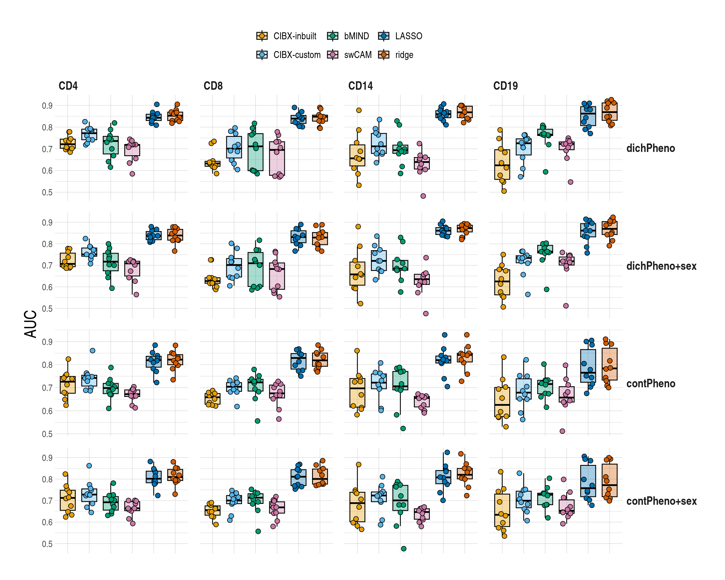

Differential gene expression (DGE) recovery. Area under curve (AUC) distributions by cell type (columns) and approach for each scenario (rows). dichPheno: simulated dichotomous phenotype; dichPheno+sex: simulated dichotomous phenotype and sex; contPheno: continous phenotype; contPheno+sex: continous phenotype and sex. Each point is a simulated phenotype, and there are ten simulated phenotypes. For each simulated phenotype, the receiver operating characteristic curve and AUC were estimated by FDR fixed at 0.05 in the observed data and varied FDRs from 0 to 1 by 0.05 in the imputed data. Box plots showed the AUC distributions, with horizontal lines from the bottom to the top for 25 %, 50 % and 75 % quantiles, respectively. inbuilt: CIBERSORTx with the inbuilt signature matrix; custom: CIBERSORTx with a custom signature matrix; bMIND: bMIND with flow fractions; swCAM: swCAM with flow fractions; LASSO/RIDGE: regularised multi-response Gaussian models.

Code

mychk_tbl <- copy(mychk)
mychk_tbl[, .N, by = c("scenarios", "celltype", "approach")]
             scenarios celltype approach  N
  1:   main.dcht.nocov      CD4  inbuilt 10
  2:   main.dcht.nocov      CD4   custom 10
  3:   main.dcht.nocov      CD4    bMIND 10
  4:   main.dcht.nocov      CD4    swCAM 10
  5:   main.dcht.nocov      CD4    LASSO 10
 ---                                       
188: common.cntn.covin     CD19   custom 10
189: common.cntn.covin     CD19    bMIND 10
190: common.cntn.covin     CD19    swCAM 10
191: common.cntn.covin     CD19    LASSO 10
192: common.cntn.covin     CD19    RIDGE 10

tbl_summary <- mychk_tbl[, list(
  Q50 = median(auc) %>% round(., 2),
  Q25 = quantile(auc, probs = 0.25) %>% round(., 2),
  Q75 = quantile(auc, probs = 0.75) %>% round(., 2)
),
by = c("scenarios", "celltype", "approach")
][
  , V1 := paste0(Q50, " (", Q25, "-", Q75, ")")
]

tbl_summary[, pheno := gsub("^main\\.|^common\\.", "", scenarios)]
tbl_summary[, scenario := str_extract(scenarios, "main|common")]

tbl_res <- dcast(
  data = tbl_summary, pheno + celltype ~ scenario + approach,
  value.var = "V1"
)

setDF(tbl_res, rownames = paste0(tbl_res$pheno, tbl_res$celltype))

pheno.order <- CJ(c("dcht", "cntn"), c("nocov", "covin"), sorted = FALSE)[, paste(V1, V2, sep = ".")]

cols.order <- CJ(c("main", "common"), V2 = expr_order, sorted = FALSE)[, paste(V1, V2, sep = "_")]

rows.order <- CJ(pheno.order, sctorder, sorted = FALSE)[, paste0(pheno.order, sctorder)]

tbl_out <- tbl_res[rows.order, c("celltype", grep("main", cols.order, value = TRUE))]
names(tbl_out) <- gsub("main_|common_", "", names(tbl_out))

kbl(
  x = tbl_out, row.names = FALSE,
  caption = "Median AUC (Q25-Q75) across 10 simulated phentoypes per cell by apparoch. **No. predicted genes vary with cell type and approaches.**"
) %>%
  kable_paper("striped", full_width = FALSE) %>%
  pack_rows("dichotomous pheno", 1, 4,
    label_row_css = "text-align: left;"
  ) %>%
  pack_rows("dichotomous pheno + sex", 5, 8) %>%
  pack_rows("continous pheno", 9, 12) %>%
  pack_rows("continous pheno + sex", 13, 16) %>%
  column_spec(column = 6:7, bold = T)

Median AUC (Q25-Q75) across 10 simulated phentoypes per cell by apparoch. **No. predicted genes vary with cell type and approaches.**
celltype	inbuilt	custom	bMIND	swCAM	LASSO	RIDGE
dichotomous pheno
CD4	0.72 (0.7-0.74)	0.77 (0.74-0.79)	0.74 (0.68-0.76)	0.72 (0.67-0.72)	0.84 (0.83-0.86)	0.85 (0.83-0.87)
CD8	0.63 (0.62-0.64)	0.7 (0.66-0.76)	0.71 (0.6-0.77)	0.69 (0.58-0.73)	0.84 (0.82-0.85)	0.85 (0.83-0.86)
CD14	0.66 (0.62-0.72)	0.71 (0.68-0.77)	0.69 (0.68-0.72)	0.64 (0.61-0.66)	0.86 (0.84-0.88)	0.87 (0.84-0.9)
CD19	0.62 (0.56-0.7)	0.73 (0.67-0.75)	0.77 (0.76-0.79)	0.72 (0.7-0.73)	0.86 (0.81-0.89)	0.87 (0.83-0.91)
dichotomous pheno + sex
CD4	0.71 (0.69-0.76)	0.75 (0.74-0.78)	0.72 (0.67-0.76)	0.71 (0.65-0.72)	0.84 (0.82-0.86)	0.84 (0.82-0.87)
CD8	0.63 (0.62-0.64)	0.7 (0.65-0.73)	0.71 (0.6-0.76)	0.68 (0.59-0.71)	0.83 (0.81-0.86)	0.83 (0.8-0.85)
CD14	0.66 (0.61-0.72)	0.72 (0.68-0.77)	0.68 (0.68-0.72)	0.64 (0.61-0.66)	0.86 (0.84-0.88)	0.87 (0.86-0.89)
CD19	0.63 (0.56-0.68)	0.73 (0.71-0.74)	0.76 (0.76-0.79)	0.72 (0.7-0.74)	0.86 (0.83-0.89)	0.87 (0.84-0.9)
continous pheno
CD4	0.73 (0.68-0.75)	0.74 (0.71-0.75)	0.7 (0.67-0.72)	0.67 (0.66-0.69)	0.82 (0.79-0.84)	0.82 (0.8-0.84)
CD8	0.66 (0.63-0.67)	0.7 (0.68-0.72)	0.72 (0.69-0.74)	0.68 (0.66-0.71)	0.83 (0.78-0.85)	0.82 (0.79-0.85)
CD14	0.7 (0.62-0.74)	0.72 (0.7-0.76)	0.71 (0.69-0.77)	0.66 (0.62-0.66)	0.82 (0.81-0.84)	0.84 (0.81-0.85)
CD19	0.63 (0.57-0.7)	0.68 (0.65-0.74)	0.72 (0.67-0.73)	0.66 (0.64-0.7)	0.76 (0.72-0.87)	0.78 (0.73-0.87)
continous pheno + sex
CD4	0.71 (0.65-0.75)	0.73 (0.7-0.75)	0.69 (0.66-0.72)	0.66 (0.65-0.7)	0.8 (0.78-0.84)	0.81 (0.79-0.84)
CD8	0.66 (0.63-0.68)	0.7 (0.69-0.72)	0.71 (0.69-0.73)	0.67 (0.64-0.69)	0.81 (0.77-0.84)	0.8 (0.78-0.85)
CD14	0.69 (0.6-0.74)	0.72 (0.69-0.74)	0.7 (0.65-0.77)	0.65 (0.61-0.66)	0.81 (0.78-0.84)	0.82 (0.8-0.85)
CD19	0.63 (0.58-0.73)	0.7 (0.67-0.74)	0.73 (0.68-0.73)	0.65 (0.64-0.7)	0.76 (0.72-0.86)	0.77 (0.72-0.87)

1.6 Fig6, simdata

Code

simdata_dir <- file.path(here::here(), "simDataRes")
simdata_dir
[1] "/rds/project/rds-csoP2nj6Y6Y/wyl37/Rbookdown/sceQTLGen/simDataRes"

sim_ids <- list.dirs(file.path(simdata_dir, "deconvInput"),
  full.names = FALSE, recursive = FALSE
)
sim_ids
 [1] "1Msim_Combatdat.160.1.100" "1Msim_Combatdat.160.1.25" 
 [3] "1Msim_Combatdat.160.1.50"  "1Msim_Combatdat.160.1.75" 
 [5] "1Msim_Combatdat.160.2.100" "1Msim_Combatdat.160.2.25" 
 [7] "1Msim_Combatdat.160.2.50"  "1Msim_Combatdat.160.2.75" 
 [9] "1Msim_Combatdat.160.3.100" "1Msim_Combatdat.160.3.25" 
[11] "1Msim_Combatdat.160.3.50"  "1Msim_Combatdat.160.3.75" 
[13] "1Msim_dat.160.1.100"       "1Msim_dat.160.1.25"       
[15] "1Msim_dat.160.1.50"        "1Msim_dat.160.1.75"       
[17] "1Msim_dat.160.2.100"       "1Msim_dat.160.2.25"       
[19] "1Msim_dat.160.2.50"        "1Msim_dat.160.2.75"       
[21] "1Msim_dat.160.3.100"       "1Msim_dat.160.3.25"       
[23] "1Msim_dat.160.3.50"        "1Msim_dat.160.3.75"       

names(sim_ids) <- sim_ids

sim_ids <- str_sort(sim_ids, numeric = TRUE)
sim_ids
 [1] "1Msim_Combatdat.160.1.25"  "1Msim_Combatdat.160.1.50" 
 [3] "1Msim_Combatdat.160.1.75"  "1Msim_Combatdat.160.1.100"
 [5] "1Msim_Combatdat.160.2.25"  "1Msim_Combatdat.160.2.50" 
 [7] "1Msim_Combatdat.160.2.75"  "1Msim_Combatdat.160.2.100"
 [9] "1Msim_Combatdat.160.3.25"  "1Msim_Combatdat.160.3.50" 
[11] "1Msim_Combatdat.160.3.75"  "1Msim_Combatdat.160.3.100"
[13] "1Msim_dat.160.1.25"        "1Msim_dat.160.1.50"       
[15] "1Msim_dat.160.1.75"        "1Msim_dat.160.1.100"      
[17] "1Msim_dat.160.2.25"        "1Msim_dat.160.2.50"       
[19] "1Msim_dat.160.2.75"        "1Msim_dat.160.2.100"      
[21] "1Msim_dat.160.3.25"        "1Msim_dat.160.3.50"       
[23] "1Msim_dat.160.3.75"        "1Msim_dat.160.3.100"      

simdata_dir
[1] "/rds/project/rds-csoP2nj6Y6Y/wyl37/Rbookdown/sceQTLGen/simDataRes"

noimpvgene <- mclapply(sim_ids, function(runid) {
  resin <- prep_dat(rid = runid, res_dir = simdata_dir)
  ## main
  mainres <- sapply(unlist(resin$iexpr, recursive = FALSE), nrow)
  ## common
  commres <- sapply(unlist(resin$icexpr, recursive = FALSE), nrow)

  data.table(
    runid = runid,
    appro = tstrsplit(names(mainres), "\\.", keep = 1L) %>% unlist(),
    celltype = tstrsplit(names(mainres), "\\.", keep = 2L) %>% unlist(),
    mainNo = mainres,
    commNo = commres[match(names(mainres), names(commres))]
  )
}, mc.cores = 6) %>% rbindlist()

Code

noimpvgene[, ":="(
  rungrp = str_remove(runid, pattern = "\\.[[:digit:]]+$"),
  trainPer = tstrsplit(runid, "\\.", keep = 4L) %>%
    unlist(),
  CombatYN = ifelse(str_detect(runid, "Combatdat"), "Y", "N")
)]

simnopredtbl <- dcast(data = noimpvgene, celltype + runid ~ appro, value.var = "mainNo")
simnopredtbl[, celltype := factor(celltype, sctorder)]
simnopredtbl[, runid := factor(runid, levels = unique(runid) %>% str_sort(., numeric = TRUE))]

setorder(simnopredtbl, celltype, runid)
setcolorder(simnopredtbl, neworder = c("runid", "celltype", expr_order))

r_idx <- apply(simnopredtbl[, ..expr_order], 1, function(x) any(x < 100)) %>% which()

kbl(x = simnopredtbl, caption = "No.predicted genes", booktabs = TRUE) %>%
  kable_paper("striped", full_width = F) %>%
  row_spec(row = r_idx, bold = TRUE)

No.predicted genes
runid	celltype	inbuilt	custom	bMIND	swCAM	LASSO	RIDGE
1Msim_Combatdat.160.1.25	CD4	3353	4776	11986	11987	11982	11646
1Msim_Combatdat.160.1.50	CD4	3272	4665	11993	11994	11913	11913
1Msim_Combatdat.160.1.75	CD4	3619	4924	11995	11996	11910	11994
1Msim_Combatdat.160.1.100	CD4	3519	4714	12005	12006	12004	11931
1Msim_Combatdat.160.2.25	CD4	2108	4347	11961	11975	11926	11972
1Msim_Combatdat.160.2.50	CD4	2853	4284	11977	11981	11979	11979
1Msim_Combatdat.160.2.75	CD4	2716	4356	11979	11981	11979	11914
1Msim_Combatdat.160.2.100	CD4	2703	4295	11973	11974	11972	11972
1Msim_Combatdat.160.3.25	CD4	3183	6160	11982	11983	11879	11707
1Msim_Combatdat.160.3.50	CD4	3502	5601	11971	11976	11942	11974
1Msim_Combatdat.160.3.75	CD4	3465	5535	11976	11981	11979	11935
1Msim_Combatdat.160.3.100	CD4	3698	5559	12461	12464	12461	12416
1Msim_dat.160.1.25	CD4	1128	4388	11977	11977	11917	11898
1Msim_dat.160.1.50	CD4	1053	4791	11981	11981	11955	11907
1Msim_dat.160.1.75	CD4	1215	4319	11992	11992	11990	11990
1Msim_dat.160.1.100	CD4	1212	4301	11996	11996	11994	11994
1Msim_dat.160.2.25	CD4	1085	4112	11983	11984	11886	11945
1Msim_dat.160.2.50	CD4	1512	4191	11998	11999	11997	11997
1Msim_dat.160.2.75	CD4	1384	4237	11997	11997	11995	11981
1Msim_dat.160.2.100	CD4	1373	4917	11986	11986	11974	11974
1Msim_dat.160.3.25	CD4	973	4691	11964	11966	11905	11855
1Msim_dat.160.3.50	CD4	1076	5242	11960	11964	11933	11928
1Msim_dat.160.3.75	CD4	1160	5215	11963	11964	11962	11949
1Msim_dat.160.3.100	CD4	2026	5225	12463	12463	12460	12460
1Msim_Combatdat.160.1.25	CD8	2595	4292	11975	11966	11924	11723
1Msim_Combatdat.160.1.50	CD8	2569	4295	11978	11966	11986	11986
1Msim_Combatdat.160.1.75	CD8	2737	4137	11986	11991	11939	11939
1Msim_Combatdat.160.1.100	CD8	3021	4235	11997	11997	11999	11999
1Msim_Combatdat.160.2.25	CD8	2638	5067	11941	11954	11886	11884
1Msim_Combatdat.160.2.50	CD8	3300	5010	11944	11978	11974	11974
1Msim_Combatdat.160.2.75	CD8	3244	4941	11953	11974	11974	11899
1Msim_Combatdat.160.2.100	CD8	3380	4850	11958	11970	11968	11968
1Msim_Combatdat.160.3.25	CD8	2626	6193	11958	11982	11976	11805
1Msim_Combatdat.160.3.50	CD8	2714	5679	11941	11975	11970	11970
1Msim_Combatdat.160.3.75	CD8	2821	5603	11943	11980	11975	11975
1Msim_Combatdat.160.3.100	CD8	2960	5563	12439	12461	12457	12457
1Msim_dat.160.1.25	CD8	2291	4780	11964	11977	11970	11970
1Msim_dat.160.1.50	CD8	2158	4107	11951	11981	11953	11974
1Msim_dat.160.1.75	CD8	2142	4735	11979	11992	11985	11985
1Msim_dat.160.1.100	CD8	2063	4695	11978	11995	11989	11972
1Msim_dat.160.2.25	CD8	1984	5045	11929	11984	11884	11855
1Msim_dat.160.2.50	CD8	1789	5240	11945	11999	11975	11975
1Msim_dat.160.2.75	CD8	1804	5091	11966	11995	11965	11971
1Msim_dat.160.2.100	CD8	1903	4493	11972	11986	11979	11964
1Msim_dat.160.3.25	CD8	1823	5582	11939	11966	11960	11855
1Msim_dat.160.3.50	CD8	1766	4154	11924	11961	11960	11960
1Msim_dat.160.3.75	CD8	1765	4215	11912	11964	11919	11960
1Msim_dat.160.3.100	CD8	1958	4293	12432	12461	12455	12455
1Msim_Combatdat.160.1.25	CD14	2730	6680	11956	11981	11985	11956
1Msim_Combatdat.160.1.50	CD14	3545	6799	11976	11993	11993	11993
1Msim_Combatdat.160.1.75	CD14	3604	6772	11981	11992	11990	11981
1Msim_Combatdat.160.1.100	CD14	3767	6838	11992	12000	12005	12005
1Msim_Combatdat.160.2.25	CD14	3098	6798	11969	11935	11923	11933
1Msim_Combatdat.160.2.50	CD14	3426	6805	11976	11959	11961	11904
1Msim_Combatdat.160.2.75	CD14	3376	6808	11975	11973	11980	11962
1Msim_Combatdat.160.2.100	CD14	3382	6909	11971	11972	11937	11919
1Msim_Combatdat.160.3.25	CD14	2845	4604	11977	11931	11924	11957
1Msim_Combatdat.160.3.50	CD14	2760	4937	11970	11926	11955	11965
1Msim_Combatdat.160.3.75	CD14	2845	4999	11976	11917	11980	11980
1Msim_Combatdat.160.3.100	CD14	3529	5265	12459	12433	12462	12462
1Msim_dat.160.1.25	CD14	3875	3467	11950	11977	11930	11976
1Msim_dat.160.1.50	CD14	4268	2135	11966	11981	11980	11980
1Msim_dat.160.1.75	CD14	4333	3987	11973	11992	11991	11979
1Msim_dat.160.1.100	CD14	4386	3989	11985	11996	11986	11995
1Msim_dat.160.2.25	CD14	3770	4915	11976	11980	11967	11983
1Msim_dat.160.2.50	CD14	4077	4553	11991	11999	11970	11979
1Msim_dat.160.2.75	CD14	4213	4750	11995	11996	11988	11989
1Msim_dat.160.2.100	CD14	4172	2656	11983	11986	11985	11985
1Msim_dat.160.3.25	CD14	4353	3073	11960	11966	11940	11941
1Msim_dat.160.3.50	CD14	4395	4008	11962	11964	11964	11948
1Msim_dat.160.3.75	CD14	4267	4040	11961	11964	11949	11944
1Msim_dat.160.3.100	CD14	4457	4207	12461	12459	12455	12455
1Msim_Combatdat.160.1.25	CD19	8	982	11924	10073	11922	11919
1Msim_Combatdat.160.1.50	CD19	55	968	11863	9961	11935	11906
1Msim_Combatdat.160.1.75	CD19	14	892	11863	9945	11946	11946
1Msim_Combatdat.160.1.100	CD19	51	927	11879	10128	11952	11952
1Msim_Combatdat.160.2.25	CD19	1	1059	11948	11381	11871	11893
1Msim_Combatdat.160.2.50	CD19	1	1095	11935	10023	11926	11904
1Msim_Combatdat.160.2.75	CD19	32	1018	11923	10167	11917	11927
1Msim_Combatdat.160.2.100	CD19	57	945	11895	8760	11910	11898
1Msim_Combatdat.160.3.25	CD19	6	86	11942	11653	11913	11932
1Msim_Combatdat.160.3.50	CD19	13	1298	11915	11364	11904	11928
1Msim_Combatdat.160.3.75	CD19	33	1342	11928	11311	11931	11901
1Msim_Combatdat.160.3.100	CD19	46	1476	12374	11824	12377	12377
1Msim_dat.160.1.25	CD19	1198	2589	11958	10689	11914	11906
1Msim_dat.160.1.50	CD19	1144	3409	11923	11183	11919	11914
1Msim_dat.160.1.75	CD19	1396	2252	11938	11159	11933	11930
1Msim_dat.160.1.100	CD19	1956	2323	11945	11578	11940	11940
1Msim_dat.160.2.25	CD19	1823	1475	11939	11887	11909	11924
1Msim_dat.160.2.50	CD19	2647	1478	11914	11992	11941	11934
1Msim_dat.160.2.75	CD19	2875	1391	11907	11961	11943	11943
1Msim_dat.160.2.100	CD19	2783	2870	11880	11973	11927	11923
1Msim_dat.160.3.25	CD19	1052	1821	11954	11370	11891	11906
1Msim_dat.160.3.50	CD19	787	2100	11939	10372	11908	11907
1Msim_dat.160.3.75	CD19	474	2085	11939	10721	11906	11913
1Msim_dat.160.3.100	CD19	2310	2124	12401	10990	12375	12366

Code

simres_f <- "simres_chunksize.rds"

if (!file.exists(simres_f)) {
  sim_pen_chunks <- lapply(seq_along(sim_ids), function(idx) {
    chunk_files <- file.path(
      simdata_dir,
      paste0("PenalisedInput/", sim_ids[idx])
    ) %>% list.files(
      pattern = "*_chunk[[:digit:]]+.rds",
      full.names = TRUE
    )

    chunk_celltypes <- str_extract(
      basename(chunk_files),
      "CD4|CD8|CD14|CD19"
    )

    chunk_s <- sapply(chunk_files, function(c_f) {
      readRDS(c_f)[["yyinput"]] %>% ncol()
    })

    data.table(celltype = chunk_celltypes, chunksize = chunk_s)
  }) %>%
    set_names(x = ., value = sim_ids) %>%
    rbindlist(., idcol = "simid")

  saveRDS(object = sim_pen_chunks, file = simres_f)
}

if (file.exists(simres_f)) {
  sim_pen_chunks <- readRDS(simres_f)
}


## no.chunks by cell type across pesudobulk data
sim_pen_chunks[,
  {
    Nchunks <- .N
    sizesmin <- min(chunksize)
    sizesmax <- max(chunksize)
    list(Nchunks, sizesmin, sizesmax)
  },
  by = c("celltype")
][match(sctorder, celltype), ]
   celltype Nchunks sizesmin sizesmax
1:      CD4    1358        4      500
2:      CD8    1306        8      498
3:     CD14    1533        3      499
4:     CD19    1180        2      497

Code

simdata_dir
[1] "/rds/project/rds-csoP2nj6Y6Y/wyl37/Rbookdown/sceQTLGen/simDataRes"

simres_f <- "simres_all.rds"

if (!file.exists(simres_f)) {
  simres_all <- lapply(sim_ids, function(runid) {
    message(runid)
    datin <- prep_dat(rid = runid, res_dir = simdata_dir)

    commonexpr <- datin$icexpr

    ## 0 genes common across methods
    if (any(sapply(datin$icexpr[[1]], nrow) == 0)) {
      k_ct <- which(sapply(datin$icexpr[[1]], nrow) != 0) %>%
        names(datin$icexpr[[1]])[.]

      commonexpr <- lapply(datin$icexpr, function(xin) {
        xin[k_ct]
      })
    }

    impvexpr_all <- list(
      main = datin$iexpr,
      common = commonexpr
    )

    observy <- datin$oexpr
    train_samps_ct <- datin$trainsamp
    sampdata <- datin$phenodata

    ## sce1: train+test in [1] & [2]
    ## sce2: test in [1] & [2]

    sce_list <- list(
      sce1 = list(tsin = train_samps_ct, testsamp = FALSE),
      sce2 = list(tsin = NULL, testsamp = FALSE)
    )

    numCores <- length(impvexpr_all) * length(sce_list)
    numCores

    cl <- makeCluster(numCores, type = "FORK")
    registerDoParallel(cl)

    aucall <- foreach(
      j = seq_along(impvexpr_all),
      .final = function(x) setNames(x, names(impvexpr_all))
    ) %:%
      foreach(
        i = seq_along(sce_list),
        .final = function(x) setNames(x, names(sce_list))
      ) %dopar% {
        tsin <- sce_list[[i]][["tsin"]]

        ttin <- sce_list[[i]][["testsamp"]]

        dat <- run_datprepfig4(
          obvexpr = observy,
          impvexpr = impvexpr_all[[j]],
          tsampct = tsin,
          phenodata = sampdata,
          dich = TRUE
        )
        ## expr ~ pheno
        res1 <- run_fig4(
          datprlst = dat,
          truesig = 0.05, testsamp = ttin
        )

        ## expr~ batch + pheno
        res2 <- run_fig4(
          datprlst = dat, truesig = 0.05,
          testsamp = ttin,
          covdata = sampdata, covid = "sample",
          covar = "batch"
        )

        list(nocov = res1, covin = res2)
      }

    stopCluster(cl)

    aucall
  })

  names(simres_all) <- sim_ids

  simresmychk <- unlist(simres_all, recursive = FALSE) %>%
    unlist(., recursive = FALSE) %>%
    unlist(., recursive = FALSE) %>%
    lapply(., "[[", "aucres") %>%
    rbindlist(l = ., idcol = "runidsce")

  saveRDS(simresmychk, file = simres_f)
}

if (file.exists(simres_f)) {
  simresmychk <- readRDS(simres_f)
}

simresmychk[, scenario := str_extract(runidsce, "main|common")]
simresmychk[, trainper := tstrsplit(simresmychk$runidsce, "\\.", keep = 4L) %>% unlist()]
simresmychk[, sce := str_extract(runidsce, "sce[1|2|3]")]
simresmychk[, pheno := str_extract(runidsce, "nocov|covin")]
simresmychk[, pheno := ifelse(grepl("Combatdat", runidsce), paste0("Cb", pheno), pheno)]

simresmychk <- simresmychk[pheno != "Cbcovin", ]

simresmychk[, ":="(
  celltype = factor(celltype, levels = sctorder),
  approach = factor(approach, levels = expr_order),
  pheno = factor(pheno,
    levels = c("nocov", "covin", "Cbnocov"),
    labels = c("cond", "batch+cond", "Combat-Seq\ncond")
  )
)]

simresmychk[, trainper := as.numeric(trainper)]

## simresmychk[, trainper := factor(trainper, levels = unique(simresmychk$trainper) %>% str_sort(., numeric = TRUE))]
## n_trainper <- nlevels(simresmychk$trainper)
## n_trainper
## shape_m <- seq(21, length.out = n_trainper) %>%
##     set_names(levels(simresmychk$trainper))

simresmychk[, approach := appro_lab[match(simresmychk$approach, names(appro_lab))]]
simresmychk[, approach := factor(approach, appro_lab)]
appro.cols.mod <- appro.cols
names(appro.cols.mod) <- appro_lab

## CIBX-inbuilt imputed < 60 genes for CD19 under Combat-Seq cond
## unstable AUCs, set the rest as NA
simresmychk[pheno == "Combat-Seq\ncond" & celltype == "CD19" & approach == "CIBX-inbuilt", ]
                                       runidsce fakedPCs     approach celltype
 1:    1Msim_Combatdat.160.1.25.main.sce1.nocov     cond CIBX-inbuilt     CD19
 2:    1Msim_Combatdat.160.1.25.main.sce2.nocov     cond CIBX-inbuilt     CD19
 3:    1Msim_Combatdat.160.1.50.main.sce1.nocov     cond CIBX-inbuilt     CD19
 4:    1Msim_Combatdat.160.1.50.main.sce2.nocov     cond CIBX-inbuilt     CD19
 5:    1Msim_Combatdat.160.1.75.main.sce1.nocov     cond CIBX-inbuilt     CD19
 6:    1Msim_Combatdat.160.1.75.main.sce2.nocov     cond CIBX-inbuilt     CD19
 7:   1Msim_Combatdat.160.1.100.main.sce1.nocov     cond CIBX-inbuilt     CD19
 8:   1Msim_Combatdat.160.1.100.main.sce2.nocov     cond CIBX-inbuilt     CD19
 9:    1Msim_Combatdat.160.2.25.main.sce1.nocov     cond CIBX-inbuilt     CD19
10:    1Msim_Combatdat.160.2.25.main.sce2.nocov     cond CIBX-inbuilt     CD19
11:    1Msim_Combatdat.160.2.50.main.sce1.nocov     cond CIBX-inbuilt     CD19
12:    1Msim_Combatdat.160.2.50.main.sce2.nocov     cond CIBX-inbuilt     CD19
13:    1Msim_Combatdat.160.2.75.main.sce1.nocov     cond CIBX-inbuilt     CD19
14:    1Msim_Combatdat.160.2.75.main.sce2.nocov     cond CIBX-inbuilt     CD19
15:   1Msim_Combatdat.160.2.100.main.sce1.nocov     cond CIBX-inbuilt     CD19
16:   1Msim_Combatdat.160.2.100.main.sce2.nocov     cond CIBX-inbuilt     CD19
17:    1Msim_Combatdat.160.3.25.main.sce1.nocov     cond CIBX-inbuilt     CD19
18:    1Msim_Combatdat.160.3.25.main.sce2.nocov     cond CIBX-inbuilt     CD19
19:    1Msim_Combatdat.160.3.50.main.sce1.nocov     cond CIBX-inbuilt     CD19
20:    1Msim_Combatdat.160.3.50.main.sce2.nocov     cond CIBX-inbuilt     CD19
21:  1Msim_Combatdat.160.3.50.common.sce1.nocov     cond CIBX-inbuilt     CD19
22:  1Msim_Combatdat.160.3.50.common.sce2.nocov     cond CIBX-inbuilt     CD19
23:    1Msim_Combatdat.160.3.75.main.sce1.nocov     cond CIBX-inbuilt     CD19
24:    1Msim_Combatdat.160.3.75.main.sce2.nocov     cond CIBX-inbuilt     CD19
25:  1Msim_Combatdat.160.3.75.common.sce1.nocov     cond CIBX-inbuilt     CD19
26:  1Msim_Combatdat.160.3.75.common.sce2.nocov     cond CIBX-inbuilt     CD19
27:   1Msim_Combatdat.160.3.100.main.sce1.nocov     cond CIBX-inbuilt     CD19
28:   1Msim_Combatdat.160.3.100.main.sce2.nocov     cond CIBX-inbuilt     CD19
29: 1Msim_Combatdat.160.3.100.common.sce1.nocov     cond CIBX-inbuilt     CD19
30: 1Msim_Combatdat.160.3.100.common.sce2.nocov     cond CIBX-inbuilt     CD19
                                       runidsce fakedPCs     approach celltype
          auc scenario trainper  sce            pheno
 1: 0.5481005     main       25 sce1 Combat-Seq\ncond
 2:        NA     main       25 sce2 Combat-Seq\ncond
 3: 0.5030582     main       50 sce1 Combat-Seq\ncond
 4: 0.4960178     main       50 sce2 Combat-Seq\ncond
 5: 0.5923738     main       75 sce1 Combat-Seq\ncond
 6: 0.9588608     main       75 sce2 Combat-Seq\ncond
 7: 0.6417989     main      100 sce1 Combat-Seq\ncond
 8: 0.5084310     main      100 sce2 Combat-Seq\ncond
 9:        NA     main       25 sce1 Combat-Seq\ncond
10:        NA     main       25 sce2 Combat-Seq\ncond
11:        NA     main       50 sce1 Combat-Seq\ncond
12:        NA     main       50 sce2 Combat-Seq\ncond
13: 0.6268437     main       75 sce1 Combat-Seq\ncond
14: 0.5205106     main       75 sce2 Combat-Seq\ncond
15: 0.5907763     main      100 sce1 Combat-Seq\ncond
16: 0.5075536     main      100 sce2 Combat-Seq\ncond
17:        NA     main       25 sce1 Combat-Seq\ncond
18:        NA     main       25 sce2 Combat-Seq\ncond
19:        NA     main       50 sce1 Combat-Seq\ncond
20:        NA     main       50 sce2 Combat-Seq\ncond
21:        NA   common       50 sce1 Combat-Seq\ncond
22:        NA   common       50 sce2 Combat-Seq\ncond
23: 0.4792505     main       75 sce1 Combat-Seq\ncond
24: 0.9679359     main       75 sce2 Combat-Seq\ncond
25:        NA   common       75 sce1 Combat-Seq\ncond
26:        NA   common       75 sce2 Combat-Seq\ncond
27: 0.5507876     main      100 sce1 Combat-Seq\ncond
28: 0.5317240     main      100 sce2 Combat-Seq\ncond
29:        NA   common      100 sce1 Combat-Seq\ncond
30:        NA   common      100 sce2 Combat-Seq\ncond
          auc scenario trainper  sce            pheno

simresmychk[pheno == "Combat-Seq\ncond" & celltype == "CD19" & approach == "CIBX-inbuilt", auc := NA]

Code

## main: varying gene sets
## common: gene sets common across approaches
## sce1: train+ test; sce2: test only
simres_pltlist <- lapply(unique(simresmychk$scenario), function(scein) {
  lapply(c("sce1", "sce2"), function(xin) {
    ggplot(
      data = simresmychk[scenario == scein & sce == xin, ],
      aes(x = trainper, y = auc, colour = approach)
    ) +
      geom_point( # aes(shape = celltype),
        alpha = 0.5, size = 1.5
      ) +
      geom_smooth(
        aes(
          group = approach,
          colour = approach,
          linetype = approach,
          fill = approach
        ),
        alpha = 0.35, se = FALSE, linewidth = 0.5
      ) +
      scale_colour_manual(values = appro.cols.mod) +
      scale_fill_manual(values = appro.cols.mod) +
      facet_grid(cols = vars(celltype), rows = vars(pheno)) +
      ylab("AUC") +
      xlab("Percentage of 80 train samples") +
      scale_x_continuous(
        breaks = seq(25, 100, by = 25),
        labels = scales::label_percent(scale = 1)
      ) +
      used_ggthemes(
        strip.text.y.right = element_text(angle = 0),
        legend.position = "top"
      )
  }) %>% set_names(., c("sce1", "sce2"))
}) %>% set_names(., unique(simresmychk$scenario))

simres_pltlist$main$sce1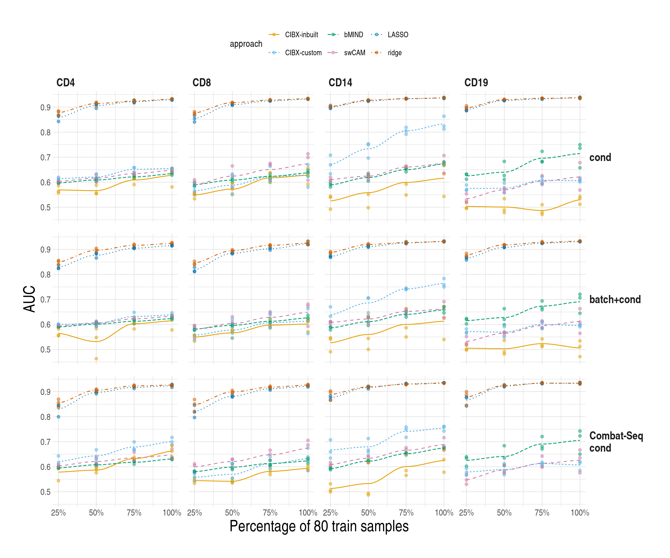

Differential gene expression (DGE) recovery. Area under curve (AUC) distributions (y-axis) across percentages of train samples (x-axis) by cell type (columns) for each scenario (rows). cond: raw synthesised read counts were used for DGE analysis of in vitro stimulation with C. albicans after 3 hours (3hCA) vs untreated (UT). batch+cond: same as cond, and included batch (V2 & V3 chemistry) as a covariate in the 3hCA-UT DGE model. Combat-seq cond: batch-corrected read counts from Combat-seq were used in DGE analysis of 3hCA vs UT. Each point is a simulation data. train and test samples + varing gene sets

Code

openxlsx::write.xlsx(
  list(
    "Fig1A" = sampdata,
    "Fig2" = pltfract_test,
    "Fig2.anno" = cordsn,
    "Fig3AB" = pedaccdsn_persub,
    "Fig3CD" = pedaccdsn,
    "Fig4" = mychk[scenario == "main",
      setdiff(names(mychk), c("scenarios", "scenario")),
      with = FALSE
    ],
    "Fig5" = simresmychk[
      scenario == "main" & sce == "sce1",
      .(approach, celltype, auc, trainper, pheno)
    ]
  ),
  file = "SourceData_mainFigures.xlsx",
  overwrite = TRUE
)

figS6 <- mychk[scenario == "common",
  setdiff(names(mychk), c("scenarios", "scenario")),
  with = FALSE
]

figS8 <- simresmychk[
  scenario == "common" & sce == "sce1",
  .(approach, celltype, auc, trainper, pheno)
]

2 Supplementary material

2.1 SupFig1, Overlap of predicted genes by approach

Overlap of predicted genes by CIBERSORTx using inbuilt (inbuilt) and our custom signatures (custom), bMIND, swCAM, LASSO and RIDGE. Predicted genes were defined as those with variations in expression across subjects. For each panel (cell type), the right bar plot indicates the numbers of predicted genes (No.Pred.Genes) by approach, and the top bar plot demonstrates No.Pred.Genes common in different combinations of approaches (black dots), but not in the grey-dot approaches, if present.

Code

col_pals <- cols4all::c4a("miscs.okabe", n = 4)

expr_scenarios <- cdata_explst$iexpr
stopifnot(names(expr_scenarios) == expr_order)
names(expr_scenarios) <- appro_lab

m_list <- lapply(seq_along(sctorder), function(idx) {
  ct <- sctorder[idx]
  Ocom <- lapply(expr_scenarios, function(dat) {
    rownames(dat[[ct]])
  })
  m1_mod <- make_comb_mat(Ocom, mode = "distinct")
  m1 <- m1_mod
  m1
})

names(m_list) <- sctorder

figS1 <- lapply(seq_along(sctorder), function(idx) {
  ct <- sctorder[idx]
  Ocom <- lapply(expr_scenarios, function(dat) {
    rownames(dat[[ct]])
  })
  max.n <- sapply(Ocom, length) %>% max()

  for (n in seq_along(Ocom)) {
    length(Ocom[[n]]) <- max.n
  }

  do.call(cbind, Ocom)
})

names(figS1) <- paste0("figS1.", sctorder)

sapply(m_list, comb_size)

m_list <- normalize_comb_mat(m_list)
sapply(m_list, comb_size)

max_set_size <- max(sapply(m_list, set_size))
max_comb_size <- max(sapply(m_list, comb_size))

ht_list <- NULL
for (i in seq_along(m_list)) {
  ht_list <- ht_list %v%
    UpSet(m_list[[i]],
      row_names_side = "left",
      row_title = paste0(names(m_list)[i]),
      row_title_gp = gpar(fontface = 2),
      row_title_rot = 0,
      set_order = names(expr_scenarios),
      comb_order = NULL,
      top_annotation = upset_top_annotation(m_list[[i]],
        ylim = c(0, max_comb_size),
        gp = gpar(fill = col_pals[2]),
        annotation_name_rot = 90,
        add_numbers = T, numbers_rot = 0
      ),
      right_annotation = upset_right_annotation(m_list[[i]],
        ylim = c(0, max_set_size),
        gp = gpar(fill = col_pals[3]),
        add_numbers = T
      )
    )
}

ht_list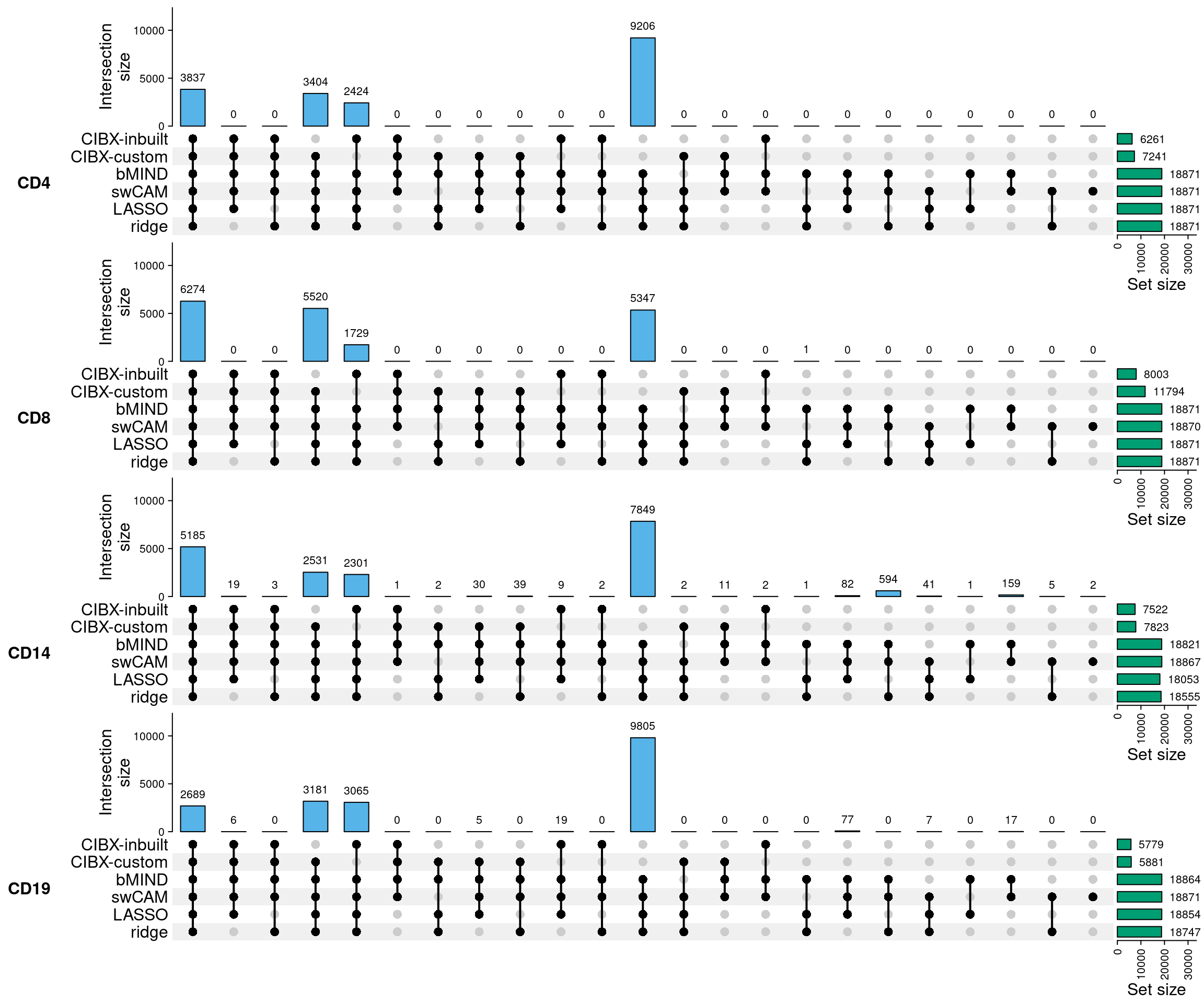

2.2 SupFig2, Correlations per subject stratified by same and different subjects

Distributions of Pearson correlations (y-axis) between observed and imputed expression across genes from the same/different subjects by cell type and approach. One estimate per subject. inbuilt: CIBERSORTx with the inbuilt signature matrix; custom: CIBERSORTx with a custom signature matrix; bMIND: bMIND with flow fractions; swCAM: swCAM with flow fractions; LASSO/RIDGE: regularised multi-response Gaussian

Code

numCores <- length(expr_order)
cl <- makeCluster(numCores, type = "FORK")
registerDoParallel(cl)

pedaccdsn_rotpersub <- foreach(j = seq_along(expr_order), .combine = "rbind") %:%

  foreach(i = seq(sctorder), .combine = "rbind") %dopar% {
    expr_scenarios <- cdata_explst$iexpr
    observy <- cdata_explst$oexpr

    sce <- expr_order[j]
    ctin <- sctorder[i]

    expr_in <- expr_scenarios[[sce]][[ctin]]
    observ_in <- observy[rownames(expr_in), colnames(expr_in)]

    ## differnt subjects
    rot <- colnames(observ_in)[c(2:ncol(observ_in), 1)]

    ## correlation across genes per subject
    resdsn <- cor(expr_in[, rot], observ_in, method = "pearson") %>% diag()

    ## rmse across genes per subject
    mse1 <- apply((observ_in - expr_in[, rot])^2, 2, mean) %>% sqrt()

    stopifnot(names(resdsn) == names(mse1))

    ## another baseline as observed expression in different subjects
    abaseline <- cor(observ_in, observ_in[, rot]) %>% diag()

    dsn1 <- data.table(
      approach = sce, celltype = ctin,
      measure_cor = resdsn,
      measure_rmse = mse1,
      avecor = abaseline
    )
    dsn1
  }

stopCluster(cl)

pedaccdsn_rotpersub[, .N, by = c("approach", "celltype")]
    approach celltype  N
 1:  inbuilt      CD4 71
 2:  inbuilt      CD8 65
 3:  inbuilt     CD14 52
 4:  inbuilt     CD19 57
 5:   custom      CD4 71
 6:   custom      CD8 65
 7:   custom     CD14 52
 8:   custom     CD19 57
 9:    bMIND      CD4 71
10:    bMIND      CD8 65
11:    bMIND     CD14 52
12:    bMIND     CD19 57
13:    swCAM      CD4 71
14:    swCAM      CD8 65
15:    swCAM     CD14 52
16:    swCAM     CD19 57
17:    LASSO      CD4 71
18:    LASSO      CD8 65
19:    LASSO     CD14 52
20:    LASSO     CD19 57
21:    RIDGE      CD4 71
22:    RIDGE      CD8 65
23:    RIDGE     CD14 52
24:    RIDGE     CD19 57
    approach celltype  N

pedaccdsn_rotpersub[, ":="(
  approach = factor(approach, levels = expr_order),
  celltype = factor(celltype, levels = sctorder)
)]


ped_a <- pedaccdsn_rotpersub[, .(approach, celltype, measure_cor)][
  , sce := "diff"
]
ped_b <- pedaccdsn_rotpersub[, .(approach, celltype, avecor)][
  , sce := "ObsDiff"
]
setnames(ped_b, old = "avecor", new = "measure_cor")

pedaccdsn_persub[, sce := "same"]

list(pedaccdsn_persub, ped_a, ped_b) %>%
  rbindlist(., fill = TRUE) %>%
  .[, sce := factor(sce, levels = c("same", "diff", "ObsDiff"))] %>%
  ggboxplot(
    data = ., x = "celltype", y = "measure_cor",
    fill = "sce",
    facet.by = "approach",
    panel.labs = list(approach = appro_lab),
    ylab = "Correlation",
    palette = "jco",
    ggtheme = used_ggthemes(
      legend.position = "top",
      legend.text = element_text(size = rel(1.2))
    )
  ) +
  labs(fill = "Subject") +
  rremove("xlab")


figS2 <- rbindlist(list(pedaccdsn_persub, ped_a, ped_b), fill = TRUE) %>%
  .[, sce := factor(sce, levels = c("same", "diff", "ObsDiff"))]

figS2[, (c("measure_rmse")) := NULL]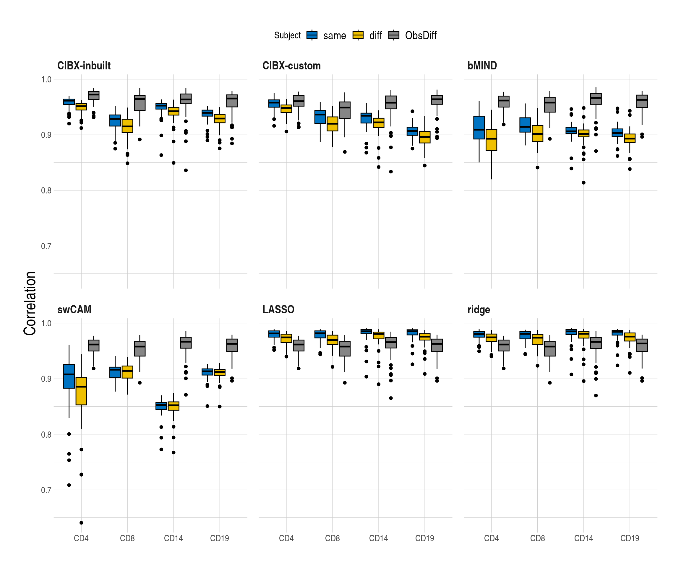

2.3 SupFig3, Common gene sets-CLUSTER data

Code

## expression from approaches
cdata_explst <- prep_dat(
  rid = "cluster",
  res_dir = data_dir,
  cluster = TRUE
)

gcommon <- lapply(sctorder, function(ctin) {
  lapply(cdata_explst$icexpr, "[[", ctin) %>%
    lapply(., rownames) %>%
    Reduce(f = intersect, x = .)
})
names(gcommon) <- sctorder

sapply(gcommon, length)
 CD4  CD8 CD14 CD19 
3837 6274 5185 2689

2.3.1 correlation & rmse per subject

Code

### predicted accuracy

observy <- cdata_explst$oexpr
expr_scenarios <- cdata_explst$icexpr

numCores <- length(expr_order)
cl <- makeCluster(numCores, type = "FORK")
registerDoParallel(cl)

pedaccdsn_persub <- foreach(i = expr_order, .combine = "rbind") %dopar% {
  run_fig3v(
    obvexpr = observy, impvexpr = expr_scenarios,
    sce = i, ct = sctorder, persub = TRUE
  ) %>%
    rbindlist()
}

stopCluster(cl)


pedaccdsn_persub[, .N, by = c("approach", "celltype")]
    approach celltype  N
 1:  inbuilt      CD4 71
 2:  inbuilt      CD8 65
 3:  inbuilt     CD14 52
 4:  inbuilt     CD19 57
 5:   custom      CD4 71
 6:   custom      CD8 65
 7:   custom     CD14 52
 8:   custom     CD19 57
 9:    bMIND      CD4 71
10:    bMIND      CD8 65
11:    bMIND     CD14 52
12:    bMIND     CD19 57
13:    swCAM      CD4 71
14:    swCAM      CD8 65
15:    swCAM     CD14 52
16:    swCAM     CD19 57
17:    LASSO      CD4 71
18:    LASSO      CD8 65
19:    LASSO     CD14 52
20:    LASSO     CD19 57
21:    RIDGE      CD4 71
22:    RIDGE      CD8 65
23:    RIDGE     CD14 52
24:    RIDGE     CD19 57
    approach celltype  N

pedaccdsn_persub[, ":="(
  approach = factor(approach, levels = expr_order),
  celltype = factor(celltype, levels = sctorder)
)][, measure_rmse := log(measure_rmse)]


measureii <- c("Correlation per subject", "log(RMSE) per subject")
names(measureii) <- c("measure_cor", "measure_rmse")

lapply(seq_along(measureii), function(idx) {
  bplt <- ggboxplot(
    data = pedaccdsn_persub,
    x = "approach",
    xlab = "",
    y = names(measureii)[idx],
    ylab = measureii[idx],
    fill = "approach",
    palette = appro.cols,
    facet.by = c("celltype")
  ) +
    facet_grid(~celltype, scales = "free")

  if (idx == 1) {
    bplt <- bplt +
      used_ggthemes(
        axis.text.x = element_blank(),
        legend.position = "none"
      )
  } else {
    bplt <- bplt +
      used_ggthemes(
        axis.text.x = element_blank(),
        legend.position = "none",
        strip.text = element_blank()
      )
  }

  bplt
})
[[1]]

[[2]]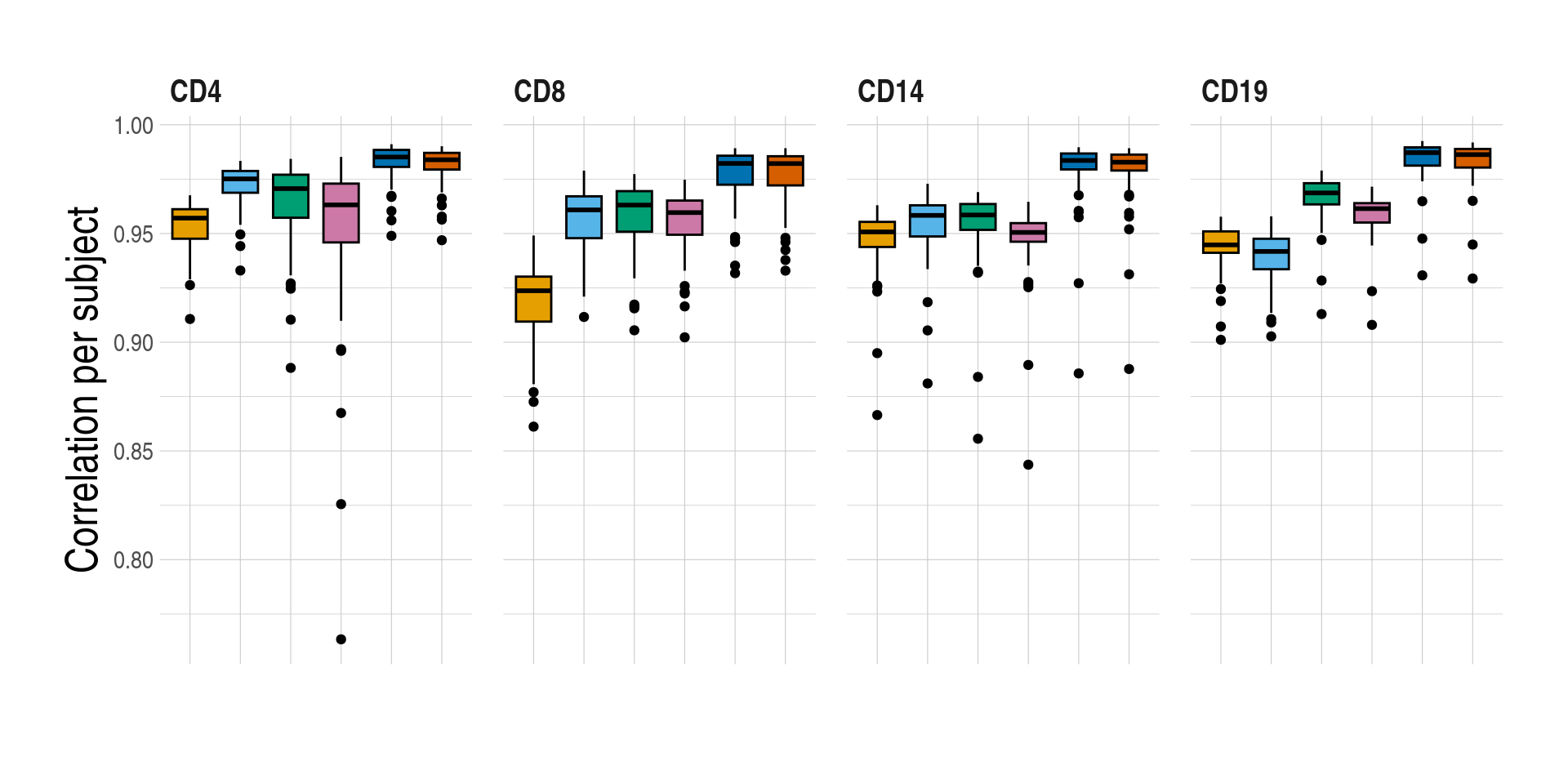

Distributions of prediction accuracy by cell type and approach. Prediction accuracy was evaluated by calculating Pearson correlation and root mean square error (RMSE) between observed and predicted cell-type expression across genes for the same subjects by cell type and approach. For each cell type, genes common across approaches were used. No. common genes are 3837 for CD4, 6274 for CD8, 5185 for CD14, and 2689 for CD19, respectively. The approaches used were: inbuilt - CIBERSORTx expression deconvolution with the inbuilt signature matrix, custom - CIBERSORTx expression deconvolution with a custom signature matrix derived from sorted cell-type expression in training samples, bMIND - bMIND expression deconvolution with flow fractions, swCAM - swCAM deconvolution with flow fractions, and LASSO/RIDGE - expression predicted from regularised multi-response Gaussian models.

2.3.2 correlation & rmse per gene

Code

numCores <- length(expr_order)
cl <- makeCluster(numCores, type = "FORK")
registerDoParallel(cl)

pedaccdsn <- foreach(i = expr_order, .combine = "rbind") %dopar% {
  run_fig3v(
    obvexpr = observy, impvexpr = expr_scenarios,
    sce = i, ct = sctorder, persub = FALSE
  ) %>%
    rbindlist()
}


stopCluster(cl)

pedaccdsn[, .N, by = c("approach", "celltype")]
    approach celltype    N
 1:  inbuilt      CD4 3837
 2:  inbuilt      CD8 6274
 3:  inbuilt     CD14 5185
 4:  inbuilt     CD19 2689
 5:   custom      CD4 3837
 6:   custom      CD8 6274
 7:   custom     CD14 5185
 8:   custom     CD19 2689
 9:    bMIND      CD4 3837
10:    bMIND      CD8 6274
11:    bMIND     CD14 5185
12:    bMIND     CD19 2689
13:    swCAM      CD4 3837
14:    swCAM      CD8 6274
15:    swCAM     CD14 5185
16:    swCAM     CD19 2689
17:    LASSO      CD4 3837
18:    LASSO      CD8 6274
19:    LASSO     CD14 5185
20:    LASSO     CD19 2689
21:    RIDGE      CD4 3837
22:    RIDGE      CD8 6274
23:    RIDGE     CD14 5185
24:    RIDGE     CD19 2689
    approach celltype    N

pedaccdsn[, ":="(
  approach = factor(approach, levels = expr_order),
  celltype = factor(celltype, levels = sctorder)
)][, measure_rmse := log(measure_rmse)]

Code

measureii <- c("Correlation per gene", "log(standardised RMSE) per gene")
names(measureii) <- c("measure_cor", "measure_rmse")

lapply(seq_along(measureii), function(idx) {
  aplt <- ggboxplot(
    data = pedaccdsn,
    x = "approach",
    xlab = "",
    y = names(measureii)[idx],
    ylab = measureii[idx],
    fill = "approach",
    palette = appro.cols,
    facet.by = c("celltype")
  ) +
    scale_fill_manual(labels = appro_lab, values = appro.cols) +
    facet_grid(~celltype, scales = "free")

  if (idx == 1) {
    aplt <- aplt + used_ggthemes(
      axis.text.x = element_blank(),
      legend.position = "none",
      strip.text = element_blank()
    )
  } else {
    aplt <- aplt + used_ggthemes(
      axis.text.x = element_blank(),
      legend.position = "top",
      strip.text = element_blank()
    )
  }


  aplt
})
[[1]]

[[2]]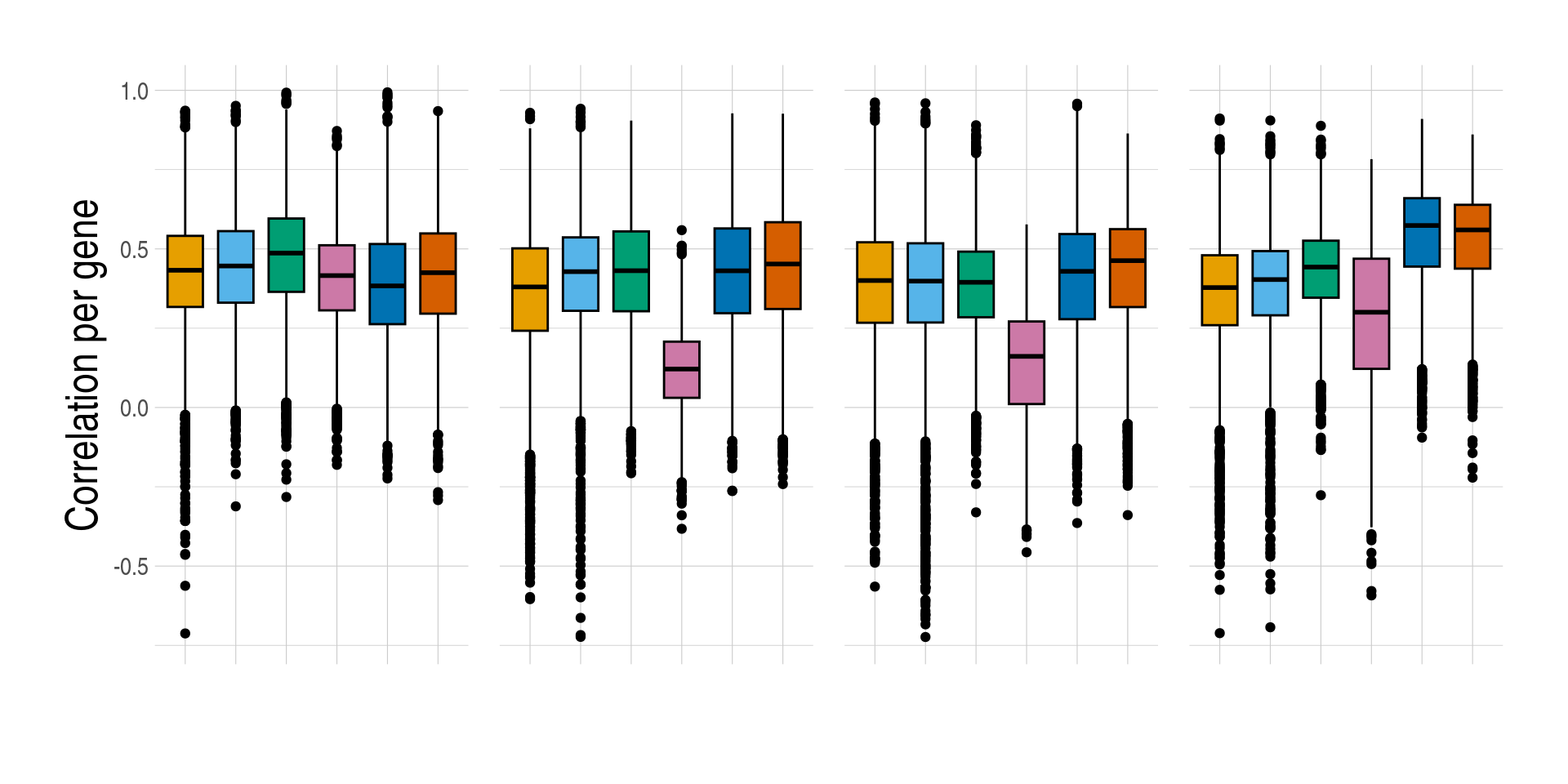

Distributions of prediction accuracy by cell type and approach. Prediction accuracy was evaluated by calculating Pearson correlation and root mean square error (RMSE) between observed and predicted cell-type expression across testing samples for each gene by cell type and approach. For each cell type, genes common across approaches were used. No. common genes are 3837 for CD4, 6274 for CD8, 5185 for CD14, and 2689 for CD19, respectively. Standardised RMSEs: RMSE/average observed expression. The approaches used were: inbuilt - CIBERSORTx expression deconvolution with the inbuilt signature matrix, custom - CIBERSORTx expression deconvolution with a custom signature matrix derived from sorted cell-type expression in training samples, bMIND - bMIND expression deconvolution with flow fractions, swCAM - swCAM deconvolution with flow fractions, and LASSO/RIDGE - expression predicted from regularised multi-response Gaussian models.

Code

figS3ab <- pedaccdsn_persub
figS3cd <- pedaccdsn

2.4 SupFig4,5-DGE recovery

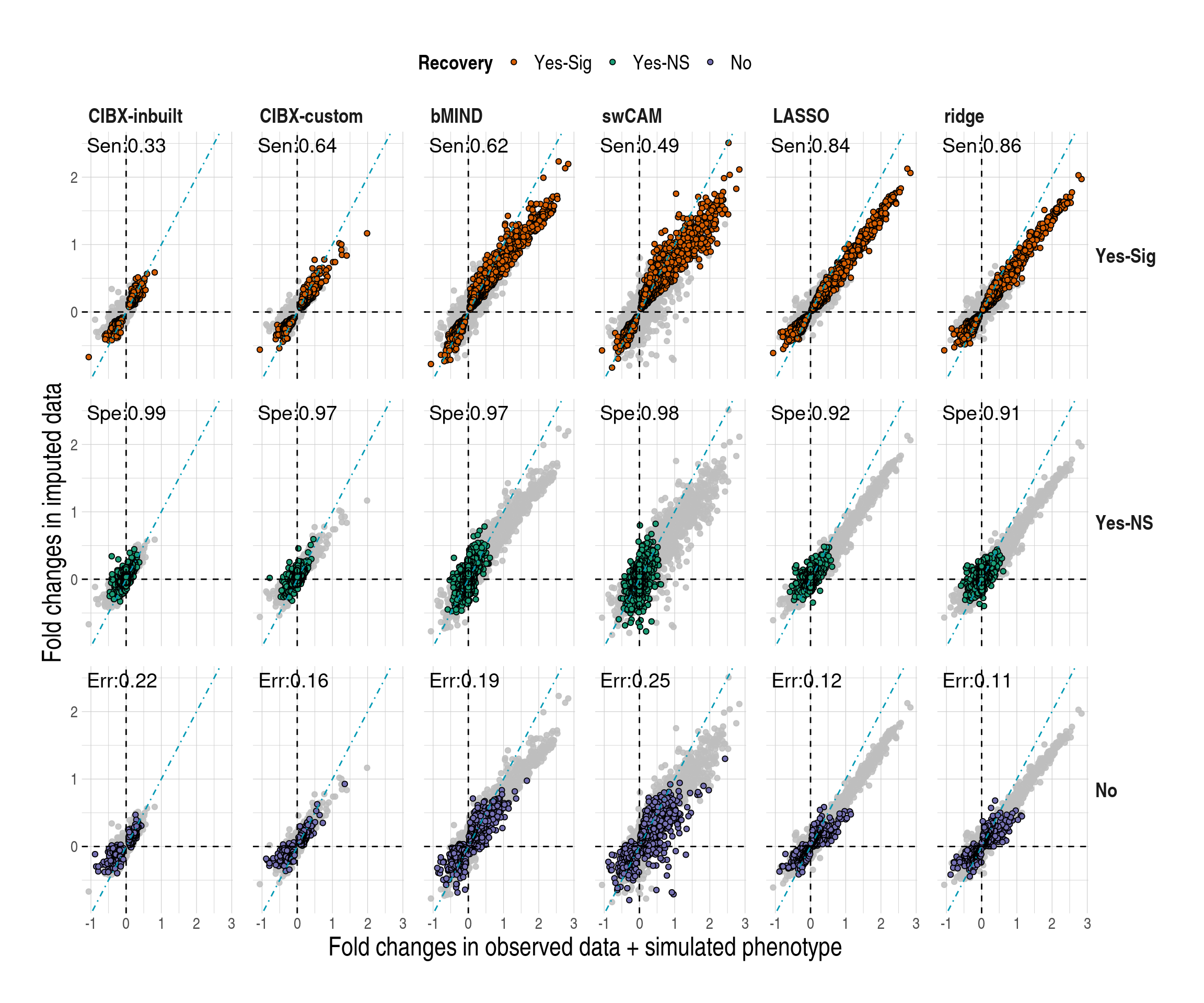
Comparisons of log\(_2\) fold changes in genes between the observed (x-axis) and imputed (y-axis) data by method (column) and by recovery status (row). DGE analysis was carried out using limma based on one of the simulated phenotypes. An FDR of 0.05 was used in both observed and imputed data here, and CD4 DGE recovery is shown. DGE results in each method (column) are the same, with coloured points for genes falling into that category of recovery status (row) and grey points for genes not belonging to the same category. Recovery status: No, Yes-NS, and Yes-Sig. Yes-Sig (sensitivity; Sen): differentially expressed genes in the observed data were also called significance in the imputed data, and the orientations of the effect sizes are the same in both data. Yes-NS (specificity; Spe): genes are called non-significance (NS) in both data. No (error; Err): misclassified genes; Err is calculated as the percentage of misclassified genes to the total number of predicted genes.

Code

degres <- copy(fig4res$dge_res) %>% setDT()
degres[, celltype := factor(celltype, levels = sctorder)]
degres[, approach := factor(approach, levels = expr_order)]

## FDR in true
fdr.thr <- 0.05

## use truecol and callmade
degres[, truecol := "0No"][adj.P.Val < fdr.thr, truecol := "1Yes"]
degres[, callmade := "0Nonsig"][
  impvadjp < fdr.thr & sign(t) == sign(impvt),
  callmade := "1Yes"
]
degres[, recovery := "No"][truecol == "1Yes" & callmade == "1Yes", recovery := "Yes-Sig"][
  truecol == "0No" & callmade == "0Nonsig", recovery := "Yes-NS"
]

## numerator
annotdsn <- degres[, .N, by = c("recovery", "fakedpheno", "approach", "celltype")]

annotdsn1 <- degres[truecol == "0No",
  {
    N_NS_obs <- .N
    list(N_NS_obs)
  },
  by = c("fakedpheno", "approach", "celltype")
][
  degres[truecol == "1Yes",
    {
      N_SIG_obs <- .N
      list(N_SIG_obs)
    },
    by = c("fakedpheno", "approach", "celltype")
  ], N_SIG_obs := i.N_SIG_obs,
  on = c("fakedpheno", "approach", "celltype")
][is.na(N_SIG_obs), N_SIG_obs := 0][
  annotdsn[recovery == "Yes-NS", ], N_recNS := i.N,
  on = c("fakedpheno", "approach", "celltype")
][
  annotdsn[recovery == "Yes-Sig", ], N_recSIG := i.N,
  on = c("fakedpheno", "approach", "celltype")
][is.na(N_recSIG), N_recSIG := 0]


tidelabfun <- function(a, b, group) {
  ## a1 <- paste0(group, ":", a, "/", b)
  a1 <- paste0(group, ":")
  if (b != 0) {
    c <- round(a / b, 2)
    ## a1 <- paste0(a1, " (", c, ")")
    a1 <- paste0(a1, c)
  }
  a1
}

annotdsn1[, ":="(
  tlab = paste0(
    tidelabfun(N_recSIG, N_SIG_obs, "Sig"), "\n",
    tidelabfun(N_recNS, N_NS_obs, "NS "), "\n",
    tidelabfun(N_recNS + N_recSIG, N_SIG_obs + N_NS_obs, "ALL")
  )

),
by = c("fakedpheno", "approach", "celltype")
]

mypaldeg <- cols4all::c4a("brewer.dark2", n = 3)
names(mypaldeg) <- c("Yes-NS", "Yes-Sig", "No")

annotdsn1[, ":="(
  tlab = paste0(
    tidelabfun(N_recSIG, N_SIG_obs, "Sen"), "\n",
    tidelabfun(N_recNS, N_NS_obs, "Spe")
  )
),
by = c("fakedpheno", "approach", "celltype")
]

mypaldeg <- cols4all::c4a("brewer.dark2", n = 3)
names(mypaldeg) <- c("Yes-NS", "Yes-Sig", "No")

## PC1 and CD4 subset
pltdsn <- degres[fakedpheno == "PC1" & celltype == "CD4", ]
pltdsn[, recovery := factor(recovery, levels = c("Yes-Sig", "Yes-NS", "No"))]

## summary of Sen & Spe, and plot lab
annodf1 <- pltdsn[, .N, by = c("approach", "recovery")]
annodf2 <- pltdsn[truecol == "1Yes", .N, by = c("approach")][, recovery := "Yes-Sig"]
annodf3 <- pltdsn[truecol == "0No", .N, by = c("approach")][, recovery := "Yes-NS"]
annodf4 <- pltdsn[, .N, by = c("approach")][, recovery := "No"]
annodf1[annodf2, Nt := i.N, on = c("approach", "recovery")]
annodf1[annodf3, Nt := i.N, on = c("approach", "recovery")]
annodf1[annodf4, Nt := i.N, on = c("approach", "recovery")]
annodf1[!is.na(Nt), pper := round(N / Nt, 2)]

annodf1[recovery == "Yes-Sig", tlab := paste0("Sen:", pper)]
annodf1[recovery == "Yes-NS", tlab := paste0("Spe:", pper)]
annodf1[recovery == "No", tlab := paste0("Err:", pper)]

kklab <- levels(pltdsn$recovery)
names(kklab) <- kklab

figS4 <- copy(pltdsn)
figS4.anno <- copy(annodf1)

ggplot(data = pltdsn, aes(x = logFC, y = impvlogFC)) +
  geom_point(data = pltdsn %>% dplyr::select(-recovery), color = "grey", alpha = 0.85) +
  geom_point(aes(fill = recovery), shape = 21) +
  geom_hline(yintercept = 0, linetype = 2, color = "black") +
  geom_vline(xintercept = 0, linetype = 2, color = "black") +
  geom_abline(
    intercept = 0, slope = 1, linetype = 4,
    color = ggsci::pal_lancet(alpha = 1)(8)[4]
  ) +
  ggrepel::geom_text_repel(
    data = annodf1,
    aes(
      x = -Inf, y = Inf,
      label = tlab
    ),
    hjust = 0, size = 5,
    min.segment.length = Inf,
    parse = FALSE
  ) +
  scale_fill_manual(values = mypaldeg) +
  facet_grid(recovery ~ approach,
    labeller = as_labeller(c(appro_lab, kklab))
  ) +
  xlab("Fold changes in observed data + simulated phenotype") +
  ylab("Fold changes in imputed data") +
  labs(fill = "Recovery") +
  used_ggthemes(
    legend.position = "top",
    axis.title = element_text(size = rel(1.2)),
    legend.text = element_text(size = rel(1.2)),
    legend.title = element_text(
      size = rel(1.2),
      face = "bold"
    ),
    strip.text.y.right = element_text(angle = 0)
  )

Receiver operating characteristic (ROC) curves and estimated area under curve (AUC) by cell type and approach based on one simulated phenotype. FDR was fixed at 0.05 in the observed data and varied from 0 to 1 by 0.05 in the imputed data.

Code

###################################################################################
## summarise the ROC curves by approach based on the first simulated phenotypes  ##
###################################################################################
## pc1 as example
pc_examp <- "PC1"

rocresall <- fig4res$rocresall

myaucs <- fig4res$aucres[fakedPCs == "PC1", ]
myaucs[, auc := round(auc, 3)]
myaucs[, name := paste(celltype, approach, sep = ".")]


appro.cols.MOD <- appro.cols[match(myaucs$approach, names(appro.cols))]
names(appro.cols.MOD) <- myaucs$name

myaucs[, ":="(
  celltype = factor(celltype, levels = sctorder),
  approach = factor(approach,
    levels = expr_order
  )
)]

myrun <- lapply(sctorder, function(ctin) {
  aucpltdsn <- lapply(rocresall[[pc_examp]][[ctin]], "[[", "rocres")
  names(aucpltdsn) <- paste0(ctin, ".", names(aucpltdsn))
  aucpltdsn
})

myrun <- unlist(myrun, recursive = FALSE)

library(pROC)
g.list <- ggroc(myrun, legacy.axes = TRUE)

kklab <- sctorder
names(kklab) <- sctorder

g.list$data$celltype <- tstrsplit(g.list$data$name, "\\.", keep = 1L) %>%
  unlist() %>%
  factor(., levels = sctorder)
g.list$data$approach <- tstrsplit(g.list$data$name, "\\.", keep = 2L) %>%
  unlist() %>%
  factor(., levels = expr_order)

g.list +
  scale_color_manual(values = appro.cols.MOD) +
  facet_grid(celltype ~ approach,
    labeller = as_labeller(c(appro_lab, kklab))
  ) +
  geom_text(
    data = myaucs,
    aes(0.75, 0.25,
      label = auc
    ),
    size = 6
  ) +
  geom_abline(
    slope = 1, intercept = 0, linetype = 2,
    colour = cols4all::c4a_na("okabe")
  ) +
  ylab("Sensitivity") +
  xlab("1-Specificity") +
  used_ggthemes(
    legend.position = "none",
    strip.text.y.right = element_text(angle = 0)
  )

figS5 <- g.list$data
figS5.anno <- myaucs[, .(approach, celltype, auc, name)]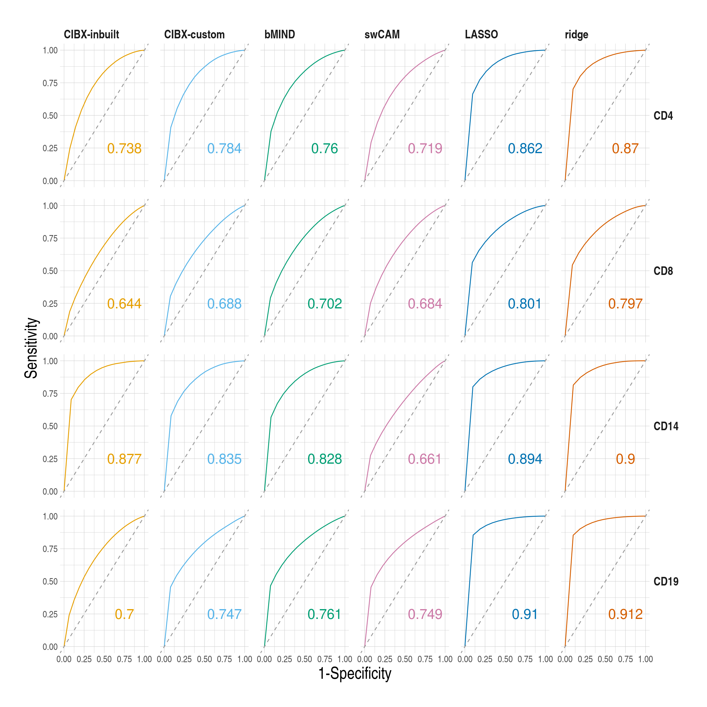

2.5 SupFig6, Train + Test samples, CLUSTER data

2.5.1 Common gene sets

Code

ggboxplot(
  data = mychk[scenario == "common", ],
  x = "approach", y = "auc", ylab = "AUC",
  palette = appro.cols,
  alpha = 0.35, fill = "approach",
  add = c("jitter"),
  add.params = list(shape = 21, size = 2.5, alpha = 1)
) +
  scale_fill_manual(labels = appro_lab, values = appro.cols) +
  facet_grid(pheno ~ celltype, scales = "free") +
  labs(fill = NULL) +
  used_ggthemes(
    axis.text.x = element_blank(),
    legend.position = "top",
    strip.text.y.right = element_text(angle = 0),
    legend.text = element_text(size = rel(1))
  ) +
  rremove("xlab")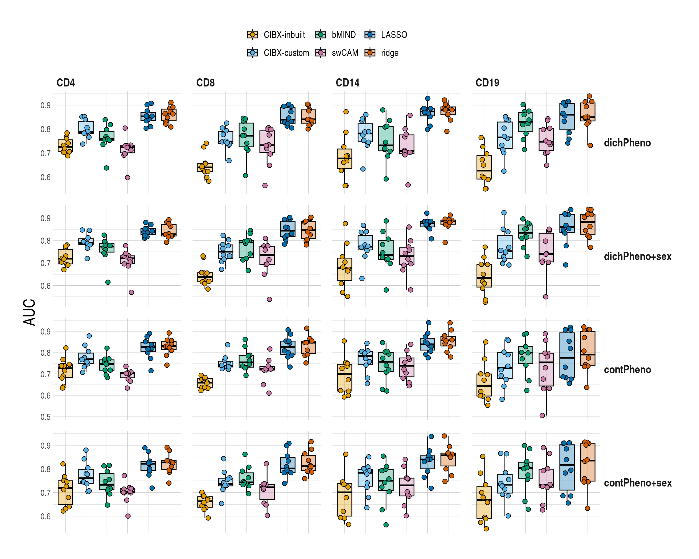

Differential gene expression (DGE) recovery. Genes common across approaches were used, and No. common genes are 3837 for CD4, 6274 for CD8, 5185 for CD14, and 2689 for CD19. Area under curve (AUC) distributions by cell type (columns) and approach for each scenario (rows). **dichPheno: simulated dichotomous phenotype; dichPheno+sex: simulated dichotomous phenotype and sex; contPheno: continous phenotype; contPheno+sex: continous phenotype and sex**. Each point is a simulated phenotype, and there are ten simulated phenotypes. For each simulated phenotype, the receiver operating characteristic curve and AUC were estimated by FDR fixed at 0.05 in the observed data and varied FDRs from 0 to 1 by 0.05 in the imputed data. Box plots showed the AUC distributions, with horizontal lines from the bottom to the top for 25 %, 50 % and 75 % quantiles, respectively. inbuilt: CIBERSORTx with the inbuilt signature matrix; custom: CIBERSORTx with a custom signature matrix; bMIND: bMIND with flow fractions; swCAM: swCAM with flow fractions; LASSO/RIDGE: regularised multi-response Gaussian models.

Code

tbl_out <- tbl_res[rows.order, c("celltype", grep("common", cols.order, value = TRUE))]
names(tbl_out) <- gsub("main_|common_", "", names(tbl_out))

kbl(
  x = tbl_out, row.names = FALSE,
  caption = "Median AUC (Q25-Q75) across 10 simulated phentoypes per cell by apparoch. **Genes common across approaches per cell type**"
) %>%
  kable_paper("striped", full_width = FALSE) %>%
  column_spec(column = 6:7, bold = T) %>%
  pack_rows("dichotomous pheno", 1, 4,
    label_row_css = "text-align: left;"
  ) %>%
  pack_rows("dichotomous pheno + sex", 5, 8) %>%
  pack_rows("continous pheno", 9, 12) %>%
  pack_rows("continous pheno + sex", 13, 16)

Median AUC (Q25-Q75) across 10 simulated phentoypes per cell by apparoch. **Genes common across approaches per cell type**
celltype	inbuilt	custom	bMIND	swCAM	LASSO	RIDGE
dichotomous pheno
CD4	0.73 (0.71-0.76)	0.79 (0.78-0.83)	0.76 (0.75-0.79)	0.72 (0.7-0.73)	0.85 (0.84-0.87)	0.86 (0.84-0.88)
CD8	0.64 (0.62-0.66)	0.75 (0.74-0.79)	0.77 (0.73-0.83)	0.73 (0.7-0.79)	0.84 (0.82-0.89)	0.84 (0.82-0.88)
CD14	0.68 (0.64-0.72)	0.78 (0.75-0.82)	0.73 (0.71-0.81)	0.71 (0.7-0.78)	0.87 (0.86-0.89)	0.88 (0.86-0.89)
CD19	0.63 (0.59-0.69)	0.77 (0.72-0.83)	0.83 (0.79-0.87)	0.75 (0.71-0.8)	0.86 (0.8-0.91)	0.85 (0.83-0.91)
dichotomous pheno + sex
CD4	0.72 (0.7-0.76)	0.79 (0.78-0.81)	0.77 (0.75-0.79)	0.72 (0.7-0.73)	0.84 (0.83-0.85)	0.83 (0.82-0.87)
CD8	0.64 (0.62-0.66)	0.75 (0.72-0.78)	0.79 (0.73-0.8)	0.74 (0.69-0.77)	0.84 (0.82-0.89)	0.85 (0.81-0.89)
CD14	0.68 (0.62-0.72)	0.77 (0.76-0.82)	0.74 (0.72-0.8)	0.73 (0.69-0.77)	0.88 (0.86-0.89)	0.89 (0.87-0.89)
CD19	0.63 (0.59-0.69)	0.75 (0.72-0.82)	0.83 (0.81-0.87)	0.74 (0.7-0.83)	0.86 (0.84-0.92)	0.88 (0.83-0.92)
continous pheno
CD4	0.73 (0.68-0.74)	0.77 (0.75-0.8)	0.75 (0.72-0.77)	0.7 (0.68-0.71)	0.83 (0.8-0.85)	0.83 (0.81-0.85)
CD8	0.66 (0.64-0.68)	0.74 (0.73-0.76)	0.75 (0.73-0.79)	0.72 (0.72-0.73)	0.83 (0.79-0.85)	0.85 (0.8-0.85)
CD14	0.7 (0.62-0.75)	0.78 (0.75-0.81)	0.76 (0.71-0.8)	0.74 (0.69-0.78)	0.84 (0.81-0.87)	0.86 (0.83-0.87)
CD19	0.64 (0.6-0.7)	0.73 (0.68-0.8)	0.8 (0.75-0.83)	0.75 (0.64-0.8)	0.78 (0.68-0.89)	0.79 (0.74-0.9)
continous pheno + sex
CD4	0.72 (0.65-0.75)	0.76 (0.74-0.8)	0.73 (0.71-0.78)	0.7 (0.7-0.72)	0.82 (0.79-0.83)	0.83 (0.8-0.83)
CD8	0.66 (0.64-0.68)	0.74 (0.73-0.76)	0.74 (0.73-0.78)	0.72 (0.67-0.73)	0.8 (0.79-0.85)	0.81 (0.79-0.86)
CD14	0.7 (0.6-0.74)	0.78 (0.73-0.8)	0.75 (0.71-0.8)	0.73 (0.69-0.76)	0.84 (0.8-0.86)	0.86 (0.81-0.87)
CD19	0.67 (0.59-0.72)	0.73 (0.7-0.78)	0.8 (0.76-0.83)	0.73 (0.72-0.8)	0.82 (0.71-0.9)	0.84 (0.75-0.91)

2.6 SupFig7, slopes

Distributions of sensitivity (y-axis) & specificity (y-axis) by cell type and approach. An FDR < 0.05 were used in both imputed and observed data. Each point is a simulated phenotype.

Code

## sen and spe across phenotypes
mychks <- copy(annotdsn1)
mychks[, Sens := N_recSIG / N_SIG_obs][
  , Spes := N_recNS / N_NS_obs
]
specresplt <- ggboxplot(
  data = mychks, x = "approach",
  y = "Spes", ylab = "Specificity",
  palette = appro.cols,
  alpha = 0.35, fill = "approach",
  add.params = list(shape = 21, size = 3, alpha = 0.8),
  add = c("jitter")
) +
  scale_fill_manual(labels = appro_lab, values = appro.cols) +
  facet_grid(~celltype, scales = "free") +
  used_ggthemes() + rremove("xlab") +
  theme(
    axis.text.x = element_blank(),
    legend.text = element_text(size = rel(1.2))
  ) +
  labs(fill = NULL)

sensresplt <- ggboxplot(
  data = mychks, x = "approach",
  y = "Sens", ylab = "Sensitivity",
  palette = appro.cols,
  alpha = 0.35, fill = "approach",
  add.params = list(shape = 21, size = 3, alpha = 0.8),
  add = c("jitter")
) +
  scale_fill_manual(labels = appro_lab, values = appro.cols) +
  facet_grid(~celltype, scales = "free") +
  used_ggthemes(
    axis.text.x = element_blank(),
    legend.text = element_text(size = rel(1.2))
  ) +
  rremove("xlab") + labs(fill = NULL)

ggarrange(sensresplt, specresplt, nrow = 2, common.legend = TRUE)

figS7a <- copy(mychks)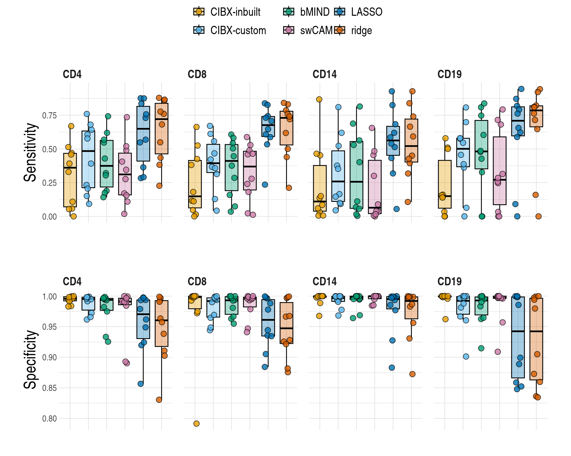

Effect sizes (logFC), standard errors (S.E.) of effect sizes, z scores of effect size between observed (x-axis) and imputed (y-axis) data based on CD4 with one simulated phenotype

Code

y <- copy(degres)
head(y)
       logFC  AveExpr        t      P.Value    adj.P.Val        B     s2post
1: 0.3554621 7.260532 8.525827 1.339332e-14 8.385557e-11 22.64075 0.06458024
2: 0.3090823 5.954265 8.394649 2.884120e-14 9.028738e-11 21.90352 0.05036503
3: 0.2993696 5.147788 8.049545 2.126368e-13 4.437730e-10 19.98378 0.05138763
4: 0.3058392 4.130806 7.938247 4.023035e-13 6.297056e-10 19.37123 0.05514713
5: 0.2602279 4.532937 7.783485 9.707277e-13 1.078018e-09 18.52517 0.04152844
6: 0.3030935 5.021438 7.772500 1.033079e-12 1.078018e-09 18.46538 0.05649601
   Nsample Ncase Ncon    impvt impvlogFC        impvp     impvadjp impvNsample
1:     151    66   85 5.287726 0.2487747 4.205486e-07 0.0002633055         151
2:     151    66   85 5.197207 0.2747704 6.374286e-07 0.0003325784         151
3:     151    66   85 4.384273 0.3168297 2.153044e-05 0.0018722509         151
4:     151    66   85 5.493173 0.3488366 1.609410e-07 0.0001439502         151
5:     151    66   85 4.416395 0.2156537 1.888024e-05 0.0017860222         151
6:     151    66   85 4.447224 0.3540465 1.663371e-05 0.0017506914         151
   impvNcase impvNcon approach celltype fakedpheno    gene truecol callmade
1:        66       85  inbuilt      CD4        PC1    CD44    1Yes     1Yes
2:        66       85  inbuilt      CD4        PC1 C1orf43    1Yes     1Yes
3:        66       85  inbuilt      CD4        PC1     VCP    1Yes     1Yes
4:        66       85  inbuilt      CD4        PC1   P2RX4    1Yes     1Yes
5:        66       85  inbuilt      CD4        PC1   NAA20    1Yes     1Yes
6:        66       85  inbuilt      CD4        PC1   PSME3    1Yes     1Yes
   recovery
1:  Yes-Sig
2:  Yes-Sig
3:  Yes-Sig
4:  Yes-Sig
5:  Yes-Sig
6:  Yes-Sig

xx <- y[fakedpheno == "PC1" & celltype == "CD4"]

library(ggplot2)
library(cowplot)
theme_set(theme_cowplot())
xx[, class := paste(truecol, callmade, sep = "/")]
xx[, se := logFC / t]
xx[, impvse := impvlogFC / impvt]
xsum <- xx[, .(n = .N, medse = median(se), medimpvse = median(impvse)), by = c("class", "approach")]
xsum[, p := n / sum(n), by = "approach"]
xsum[order(approach, class)]
           class approach    n      medse  medimpvse           p
 1:  0No/0Nonsig  inbuilt 4187 0.05508787 0.05873184 0.668743012
 2:     0No/1Yes  inbuilt   27 0.06178480 0.05758701 0.004312410
 3: 1Yes/0Nonsig  inbuilt 1372 0.05195210 0.05968275 0.219134324
 4:    1Yes/1Yes  inbuilt  675 0.05002479 0.05390566 0.107810254
 5:  0No/0Nonsig   custom 4294 0.05983496 0.05406578 0.593012015
 6:     0No/1Yes   custom  122 0.06114711 0.05215159 0.016848502
 7: 1Yes/0Nonsig   custom 1011 0.05544873 0.05477584 0.139621599
 8:    1Yes/1Yes   custom 1814 0.05195309 0.04837343 0.250517884
 9:  0No/0Nonsig    bMIND 9844 0.05656370 0.07044463 0.521646972
10:     0No/1Yes    bMIND  253 0.05715402 0.06521827 0.013406815
11: 1Yes/0Nonsig    bMIND 3340 0.05657640 0.07587389 0.176991150
12:    1Yes/1Yes    bMIND 5434 0.05345500 0.06754613 0.287955063
13:  0No/0Nonsig    swCAM 9940 0.05655989 0.08271920 0.526734142
14:     0No/1Yes    swCAM  157 0.05816015 0.07310080 0.008319644
15: 1Yes/0Nonsig    swCAM 4477 0.05538832 0.10034547 0.237242330
16:    1Yes/1Yes    swCAM 4297 0.05354609 0.09459480 0.227703884
17:  0No/0Nonsig    LASSO 9286 0.05643993 0.04478155 0.492077791
18:     0No/1Yes    LASSO  811 0.05817531 0.04490354 0.042975995
19: 1Yes/0Nonsig    LASSO 1443 0.05524053 0.04429984 0.076466536
20:    1Yes/1Yes    LASSO 7331 0.05416448 0.04387849 0.388479678
21:  0No/0Nonsig    RIDGE 9196 0.05632371 0.04528211 0.487308569
22:     0No/1Yes    RIDGE  901 0.05933682 0.04601117 0.047745218
23: 1Yes/0Nonsig    RIDGE 1240 0.05582991 0.04509011 0.065709289
24:    1Yes/1Yes    RIDGE 7534 0.05411614 0.04438538 0.399236924
           class approach    n      medse  medimpvse           p

Distributions of r-squared (Rsq, y-axis) of imputed log\(_{2}\) fold changes (FC) regression on observed effect sizes by approach.
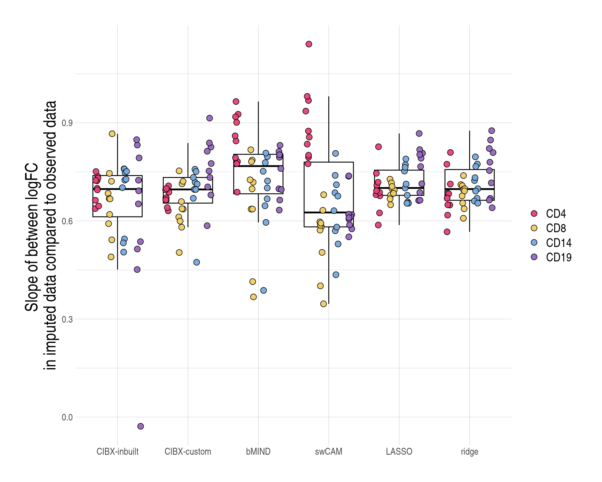
Distributions of slopes (y-axis) of imputed log\(_{2}\) fold changes (FC) regression on observed effect sizes by approach. Each point is a simulated phenotype, coloured by cell type.

Code

library(magrittr)
calc_rsq <- function(x, y) {
  summ <- lm(y ~ x) %>% summary()
  summ$r.squared
}
calc_slope <- function(x, y) {
  cf <- lm(y ~ x - 1) %>% coef()
}


ysum <- y[, .(logFC_rsq = calc_rsq(logFC, impvlogFC), logFC_slope = calc_slope(logFC, impvlogFC)),
  by = c("approach", "fakedpheno", "celltype")
]

## colors for cell type
ctfrat.pal <- friend11[seq(length(sctorder))]

## plot b
ysum[, approach := factor(approach,
  levels = expr_order,
  labels = appro_lab
)]

ggboxplot(
  data = ysum, x = "approach",
  y = "logFC_rsq",
  palette = ctfrat.pal,
  ylab = "Rsq between logFC\nin imputed and observed data",
  add = "jitter",
  add.params = list(
    fill = "celltype",
    alpha = 0.95, shape = 21,
    size = 3
  ),
  ggtheme = used_ggthemes(
    legend.text = element_text(size = rel(1.2))
  )
) +
  labs(fill = NULL) + rremove("xlab")


## plot c

ggboxplot(
  data = ysum, x = "approach",
  y = "logFC_slope",
  ylab = "Slope of between logFC \nin imputed data compared to observed data",
  palette = ctfrat.pal,
  add = "jitter",
  add.params = list(fill = "celltype", alpha = 0.95, shape = 21, size = 3),
  ggtheme = used_ggthemes(legend.text = element_text(size = rel(1.2)))
) +
  labs(fill = NULL) +
  rremove("xlab")

figS7bc <- copy(ysum)

## mean logFC slope across simulated phentoypes by approach and cell type
ysumres <- ysum[,
  {
    xx <- round(mean(logFC_slope), 2)
  },
  by = c("approach", "celltype")
]

## mean logFC slop across cell types by approach
ysumres[,
  {
    xxmin <- range(V1)[1]
    xxmax <- range(V1)[2]
    list(xxmin, xxmax)
  },
  by = "approach"
]
       approach xxmin xxmax
1: CIBX-inbuilt  0.60  0.70
2:  CIBX-custom  0.64  0.76
3:        bMIND  0.66  0.85
4:        swCAM  0.55  0.90
5:        LASSO  0.69  0.76
6:        ridge  0.68  0.76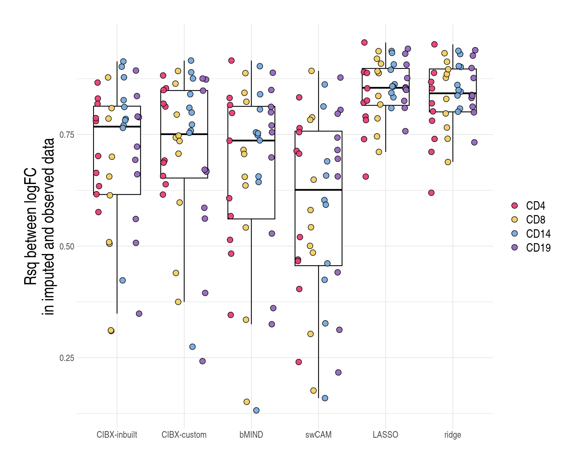

2.7 SupFig8, AUCs in pseudo datasets based on common gene sets

Code

simres_pltlist$common$sce1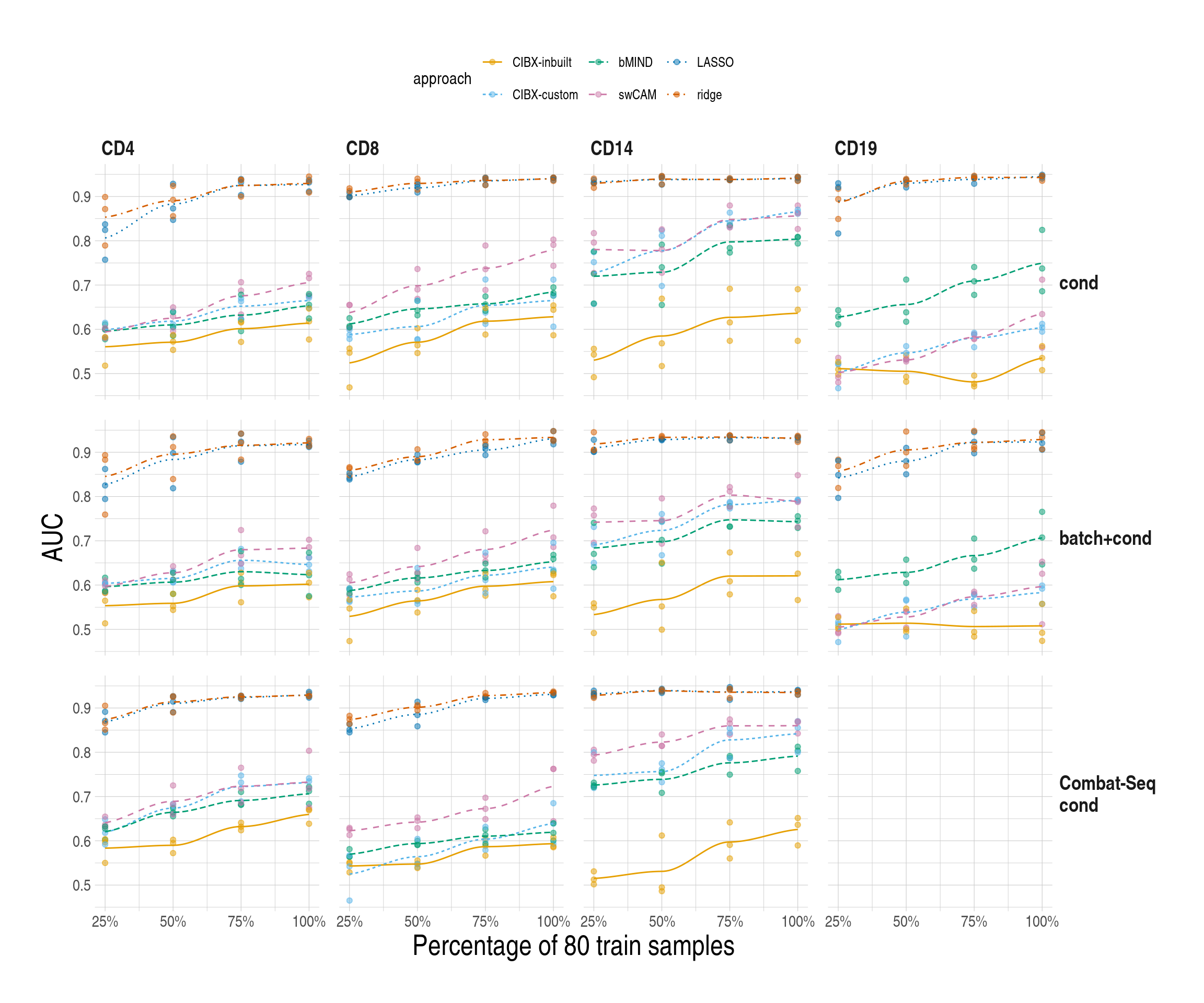

2.8 SupFig9, SupTab2, SupTab3

Code

## cluster data
proj_dir <- here::here()
proj_dir
[1] "/rds/project/rds-csoP2nj6Y6Y/wyl37/Rbookdown/sceQTLGen"

aa_files <- list.files(file.path(proj_dir, "CLUSTERdeconRes/workflowInfo"),
  "pipeline_trace*",
  full.names = TRUE
)

aadata <- lapply(aa_files, fread) %>% set_names(., basename(aa_files))

lapply(aadata, nrow)
$`pipeline_trace_2024-10-12_23-09-13.txt`
[1] 2

$`pipeline_trace_2024-10-12_23-34-29.txt`
[1] 622

$`pipeline_trace_2024-10-16_18-31-30.txt`
[1] 13

$`pipeline_trace_2024-10-16_18-39-21.txt`
[1] 5

## pipeline_trace_2024-10-12_23-34-29.txt: full run, but CIBX ran on 4 cpus
## pipeline_trace_2024-10-16_18-39-21.txt; rerun CIBX with 8 cpus

nextflowlog <- aadata[["pipeline_trace_2024-10-12_23-34-29.txt"]][!(name %in% aadata[["pipeline_trace_2024-10-16_18-39-21.txt"]]$name), ] %>%
  rbind(aadata[["pipeline_trace_2024-10-16_18-39-21.txt"]], .)

nextflowlog[, .N] # 622
[1] 622
nextflowlog <- nextflowlog[status != "FAILED", ]
nextflowlog[, .N] # 622
[1] 622

## check if realtime ==0
stopifnot(all(vtimesec(nextflowlog$realtime) != 0))

## memory units in the log
stringr::str_extract_all(nextflowlog$vmem, "[[:alpha:]]+$") |>
  unique() |>
  unlist()
[1] "MB" "GB"

## check if memory format not captured by default
nextflowlog[!stringr::str_detect(nextflowlog$vmem, "[[:alpha:]]+$")]
Empty data.table (0 rows and 17 cols): task_id,name,tag,status,exit,realtime...

stopifnot(all(!is.na(vmem.usage(nextflowlog$vmem))))

## unique process
uni_procs <- stringr::str_extract(nextflowlog$name, "[[:alnum:]]+") |> unique()
uni_procs
[1] "ZENODO"       "PREPCLUSTER"  "cibxrun"      "runSWCAM"     "runBMIND"    
[6] "runPenalised"

nextflowlog[grepl(paste0(uni_procs[1:2], collapse = "|"), name), .N] # 2
[1] 2

## exclude data prep steps
nextflowlog <- nextflowlog[!(tag %in% c("zenodo", "prepcluster")), ]
nextflowlog$trainper <- 100
nextflowlog$simdataid <- "cluster"


nextflowlog[grep("^cibxrun:LM22DECONVRUN", name), approach := "inbuilt"]
nextflowlog[grep("^cibxrun:DECONVRUN[[:space:]]", name), approach := "custom"]
nextflowlog[grep("^runBMIND:BMIND[[:space:]]", name), approach := "bMIND"]
nextflowlog[grep("^runSWCAM:SWCAM", name), approach := "swCAM"]
nextflowlog[grep("^runPenalised:PREPCHUNK", name), approach := "chunkprep"]
nextflowlog[grepl("^runPenalised", name) & grepl("lasso", tag), approach := "LASSO"]
nextflowlog[grepl("^runPenalised", name) & grepl("ridge", tag), approach := "RIDGE"]

nextflowlog[, table(approach)]
approach
    bMIND chunkprep    custom   inbuilt     LASSO     RIDGE     swCAM 
        1         4         1         1       304       304         2 

## na for fraction deconvolution or gene signature
nextflowlog[is.na(approach), name]
[1] "cibxrun:DECONVRUNGS (CIBXgs_cluster)"            
[2] "runSWCAM:DEBCAMFRACTS80 (debCAMfracts80_cluster)"
[3] "runBMIND:BMINDFRACT (bmindrunfract_cluster)"     

expr_order %in% nextflowlog$approach
[1] TRUE TRUE TRUE TRUE TRUE TRUE

rundata4plt <- lapply(expr_order, function(appin) {
  nextflowlog[approach == appin, ][,
    {
      ncpu <- unique(cpus) %>% paste0(., collapse = "/")
      cputimes <- sum(vtimesec(realtime) / 60) %>% round(., 2)
      memt <- median(vmem.usage(vmem) / 1024) %>% round(., 2)
      list(ncpu, cputimes, memt)
    },
    by = c("simdataid", "trainper")
  ]
}) %>%
  set_names(., expr_order) %>%
  rbindlist(., idcol = "approach")

## per chunk cpu time & memory for LASSO and ridge

expr_order[5:6]
[1] "LASSO" "RIDGE"

cluster_perchunk <- lapply(expr_order[5:6], function(appin) {
  nextflowlog[approach == appin, ][,
    {
      ncpu <- unique(cpus) %>% paste0(., collapse = "/")
      cputimes <- vtimesec(realtime) / 60
      memt <- vmem.usage(vmem) / 1024
      nchunk <- .N

      Q50c <- median(cputimes) %>% round(., 2)

      Q2575c <- quantile(cputimes, c(0.25, 0.75)) %>%
        round(., 2) %>%
        paste0(., collapse = ",")

      Q50m <- median(memt) %>% round(., 2)

      Q2575m <- quantile(memt, c(0.25, 0.75)) %>%
        round(., 2) %>%
        paste0(., collapse = ",")

      list(ncpu,
        nchunk,
        cputimes_pchunk = paste0(Q50c, " (", Q2575c, ")"),
        memt_pchunk = paste0(Q50m, " (", Q2575m, ")")
      )
    },
    by = c("simdataid", "trainper")
  ]
}) %>%
  set_names(., expr_order[5:6]) %>%
  rbindlist(., idcol = "approach")

rundata4plt[cluster_perchunk, Nchunks := i.nchunk, on = "approach"]
rundata4plt[cluster_perchunk, ":="(
  cpu_perchunk = i.cputimes_pchunk,
  mem_perchunk = i.memt_pchunk
), on = "approach"]

rundata4plt[, trainper := as.numeric(trainper)]

rundata4plt[, approach := appro_lab[match(rundata4plt$approach, names(appro_lab))]]

rundata4plt[, approach := factor(approach, appro_lab)]

appro.cols.mod <- appro.cols
names(appro.cols.mod) <- appro_lab

##

## cpu time
cluster_cputime <- rundata4plt[, tstrsplit(cputimes, " ", keep = 1L) %>% unlist() %>% as.numeric()]
cluster_cputime
[1]    8.80    4.45   12.00 1713.13  624.22 2928.45
## relative to CIBX
(cluster_cputime / cluster_cputime[2]) %>% round(., 2)
[1]   1.98   1.00   2.70 384.97 140.27 658.08

## mem
cluster_mem <- rundata4plt[, tstrsplit(memt, " ", keep = 1L) %>% unlist() %>% as.numeric()]
cluster_mem
[1] 11.00  5.50  1.80  2.95 16.70 58.50
## relative to CIBX
(cluster_mem / cluster_mem[2]) %>% round(., 2)
[1]  2.00  1.00  0.33  0.54  3.04 10.64

Code

setdiff(names(rundata4plt), c("simdataid", "trainper")) %>%
  rundata4plt[, ., with = FALSE] %>%
  kable(., caption = "resource usage metrics for the CLUSTER data")

resource usage metrics for the CLUSTER data
approach	ncpu	cputimes	memt	Nchunks	cpu_perchunk	mem_perchunk
CIBX-inbuilt	8	8.80	11.00	NA	NA	NA
CIBX-custom	8	4.45	5.50	NA	NA	NA
bMIND	4	12.00	1.80	NA	NA	NA
swCAM	10/1	1713.13	2.95	NA	NA	NA
LASSO	1	624.22	16.70	304	1.84 (1.23,2.73)	16.7 (11.7,24.8)
ridge	1	2928.45	58.50	304	8.85 (6.09,12.78)	58.5 (39.18,81.22)

2.9 resource usage metrics for simdata

3 simulation data (N=160 samples) x Combat-seq (Yes/No) x training percentage (25, 50, 75, 100)

Code

## simData
proj_dir <- here::here()
proj_dir
[1] "/rds/project/rds-csoP2nj6Y6Y/wyl37/Rbookdown/sceQTLGen"

## runlog
nextflowlog <- file.path(
  proj_dir,
  "simDataRes/workflowInfo/pipeline_trace_2024-10-12_22-15-21.txt"
) %>% fread()

nextflowlog[, .N] # 11073
[1] 11073
nextflowlog <- nextflowlog[status != "FAILED", ]
nextflowlog[, .N] # 11073
[1] 11073

## check if realtime ==0
stopifnot(all(vtimesec(nextflowlog$realtime) != 0))

## memory units in the log
stringr::str_extract_all(nextflowlog$vmem, "[[:alpha:]]+$") |>
  unique() |>
  unlist()
[1] "GB" "MB"

## check if memory format not captured by default
nextflowlog[!stringr::str_detect(nextflowlog$vmem, "[[:alpha:]]+$")]
Empty data.table (0 rows and 17 cols): task_id,name,tag,status,exit,realtime...

stopifnot(all(!is.na(vmem.usage(nextflowlog$vmem))))

## unique process
uni_procs <- stringr::str_extract(nextflowlog$name, "[[:alnum:]]+") |> unique()
uni_procs
[1] "PREPSCEQTL"     "CBATSIMDATA"    "SIMDATA"        "SIMDECONVINPUT"
[5] "runSWCAM"       "cibxrun"        "runBMIND"       "runPenalised"  

nextflowlog[grepl(paste0(uni_procs[1:4], collapse = "|"), name), .N] # 31
[1] 31
## tag="-" for data prep steps
nextflowlog[tag == "-", name] %>% length()
[1] 31

## exclude data prep steps
nextflowlog <- nextflowlog[tag != "-", ]
nextflowlog$trainper <- str_extract(nextflowlog$tag, "[[:digit:]]+$")
nextflowlog$simdataid <- str_extract(nextflowlog$tag, "1Msim.+$")
stopifnot(all(!is.na(nextflowlog$simdataid)))

nextflowlog[grep("^cibxrun:LM22DECONVRUN", name), approach := "inbuilt"]
nextflowlog[grep("^cibxrun:DECONVRUN[[:space:]]", name), approach := "custom"]
nextflowlog[grep("^runBMIND:BMIND[[:space:]]", name), approach := "bMIND"]
nextflowlog[grep("^runSWCAM:SWCAM", name), approach := "swCAM"]
nextflowlog[grep("^runPenalised:PREPCHUNK", name), approach := "chunkprep"]
nextflowlog[grepl("^runPenalised", name) & grepl("lasso", tag), approach := "LASSO"]
nextflowlog[grepl("^runPenalised", name) & grepl("ridge", tag), approach := "RIDGE"]

nextflowlog[, table(approach)]
approach
    bMIND chunkprep    custom   inbuilt     LASSO     RIDGE     swCAM 
       24        96        24        24      5377      5377        48 

## na for fraction deconvolution or gene signature
nextflowlog[is.na(approach), name]
 [1] "runSWCAM:DEBCAMFRACTS80 (debCAMfracts80_1Msim_Combatdat.160.2.50)" 
 [2] "runSWCAM:DEBCAMFRACTS80 (debCAMfracts80_1Msim_dat.160.1.75)"       
 [3] "runSWCAM:DEBCAMFRACTS80 (debCAMfracts80_1Msim_Combatdat.160.3.100)"
 [4] "runSWCAM:DEBCAMFRACTS80 (debCAMfracts80_1Msim_Combatdat.160.1.75)" 
 [5] "cibxrun:DECONVRUNGS (CIBXgs_1Msim_Combatdat.160.3.50)"             
 [6] "runSWCAM:DEBCAMFRACTS80 (debCAMfracts80_1Msim_dat.160.2.75)"       
 [7] "runSWCAM:DEBCAMFRACTS80 (debCAMfracts80_1Msim_Combatdat.160.2.100)"
 [8] "runSWCAM:DEBCAMFRACTS80 (debCAMfracts80_1Msim_dat.160.2.25)"       
 [9] "cibxrun:DECONVRUNGS (CIBXgs_1Msim_Combatdat.160.3.100)"            
[10] "runSWCAM:DEBCAMFRACTS80 (debCAMfracts80_1Msim_dat.160.3.25)"       
[11] "runSWCAM:DEBCAMFRACTS80 (debCAMfracts80_1Msim_dat.160.2.50)"       
[12] "runSWCAM:DEBCAMFRACTS80 (debCAMfracts80_1Msim_dat.160.1.25)"       
[13] "cibxrun:DECONVRUNGS (CIBXgs_1Msim_Combatdat.160.2.50)"             
[14] "runSWCAM:DEBCAMFRACTS80 (debCAMfracts80_1Msim_Combatdat.160.1.50)" 
[15] "runSWCAM:DEBCAMFRACTS80 (debCAMfracts80_1Msim_Combatdat.160.3.25)" 
[16] "runSWCAM:DEBCAMFRACTS80 (debCAMfracts80_1Msim_Combatdat.160.1.25)" 
[17] "runSWCAM:DEBCAMFRACTS80 (debCAMfracts80_1Msim_Combatdat.160.3.50)" 
[18] "runSWCAM:DEBCAMFRACTS80 (debCAMfracts80_1Msim_Combatdat.160.2.25)" 
[19] "runSWCAM:DEBCAMFRACTS80 (debCAMfracts80_1Msim_dat.160.3.75)"       
[20] "runSWCAM:DEBCAMFRACTS80 (debCAMfracts80_1Msim_dat.160.3.100)"      
[21] "runSWCAM:DEBCAMFRACTS80 (debCAMfracts80_1Msim_dat.160.1.100)"      
[22] "runBMIND:BMINDFRACT (bmindrunfract_1Msim_Combatdat.160.3.50)"      
[23] "runSWCAM:DEBCAMFRACTS80 (debCAMfracts80_1Msim_Combatdat.160.1.100)"
[24] "runSWCAM:DEBCAMFRACTS80 (debCAMfracts80_1Msim_Combatdat.160.2.75)" 
[25] "runBMIND:BMINDFRACT (bmindrunfract_1Msim_Combatdat.160.2.50)"      
[26] "cibxrun:DECONVRUNGS (CIBXgs_1Msim_Combatdat.160.1.100)"            
[27] "cibxrun:DECONVRUNGS (CIBXgs_1Msim_dat.160.2.25)"                   
[28] "runSWCAM:DEBCAMFRACTS80 (debCAMfracts80_1Msim_dat.160.3.50)"       
[29] "cibxrun:DECONVRUNGS (CIBXgs_1Msim_dat.160.1.75)"                   
[30] "runSWCAM:DEBCAMFRACTS80 (debCAMfracts80_1Msim_dat.160.1.50)"       
[31] "cibxrun:DECONVRUNGS (CIBXgs_1Msim_dat.160.3.25)"                   
[32] "cibxrun:DECONVRUNGS (CIBXgs_1Msim_Combatdat.160.2.100)"            
[33] "runBMIND:BMINDFRACT (bmindrunfract_1Msim_Combatdat.160.3.100)"     
[34] "runSWCAM:DEBCAMFRACTS80 (debCAMfracts80_1Msim_dat.160.2.100)"      
[35] "runSWCAM:DEBCAMFRACTS80 (debCAMfracts80_1Msim_Combatdat.160.3.75)" 
[36] "cibxrun:DECONVRUNGS (CIBXgs_1Msim_dat.160.2.75)"                   
[37] "runBMIND:BMINDFRACT (bmindrunfract_1Msim_Combatdat.160.1.100)"     
[38] "cibxrun:DECONVRUNGS (CIBXgs_1Msim_Combatdat.160.1.25)"             
[39] "cibxrun:DECONVRUNGS (CIBXgs_1Msim_Combatdat.160.2.25)"             
[40] "cibxrun:DECONVRUNGS (CIBXgs_1Msim_Combatdat.160.3.25)"             
[41] "cibxrun:DECONVRUNGS (CIBXgs_1Msim_dat.160.2.50)"                   
[42] "runBMIND:BMINDFRACT (bmindrunfract_1Msim_dat.160.1.75)"            
[43] "runBMIND:BMINDFRACT (bmindrunfract_1Msim_Combatdat.160.2.100)"     
[44] "cibxrun:DECONVRUNGS (CIBXgs_1Msim_dat.160.3.100)"                  
[45] "runBMIND:BMINDFRACT (bmindrunfract_1Msim_Combatdat.160.1.25)"      
[46] "runBMIND:BMINDFRACT (bmindrunfract_1Msim_dat.160.3.25)"            
[47] "runBMIND:BMINDFRACT (bmindrunfract_1Msim_dat.160.2.75)"            
[48] "runBMIND:BMINDFRACT (bmindrunfract_1Msim_dat.160.2.25)"            
[49] "runBMIND:BMINDFRACT (bmindrunfract_1Msim_Combatdat.160.3.25)"      
[50] "runBMIND:BMINDFRACT (bmindrunfract_1Msim_dat.160.2.50)"            
[51] "cibxrun:DECONVRUNGS (CIBXgs_1Msim_dat.160.3.50)"                   
[52] "cibxrun:DECONVRUNGS (CIBXgs_1Msim_dat.160.1.50)"                   
[53] "cibxrun:DECONVRUNGS (CIBXgs_1Msim_dat.160.1.25)"                   
[54] "cibxrun:DECONVRUNGS (CIBXgs_1Msim_Combatdat.160.2.75)"             
[55] "cibxrun:DECONVRUNGS (CIBXgs_1Msim_Combatdat.160.1.75)"             
[56] "runBMIND:BMINDFRACT (bmindrunfract_1Msim_Combatdat.160.2.25)"      
[57] "cibxrun:DECONVRUNGS (CIBXgs_1Msim_Combatdat.160.1.50)"             
[58] "runBMIND:BMINDFRACT (bmindrunfract_1Msim_dat.160.3.100)"           
[59] "runBMIND:BMINDFRACT (bmindrunfract_1Msim_dat.160.3.50)"            
[60] "runBMIND:BMINDFRACT (bmindrunfract_1Msim_Combatdat.160.1.75)"      
[61] "runBMIND:BMINDFRACT (bmindrunfract_1Msim_Combatdat.160.2.75)"      
[62] "runBMIND:BMINDFRACT (bmindrunfract_1Msim_Combatdat.160.1.50)"      
[63] "cibxrun:DECONVRUNGS (CIBXgs_1Msim_dat.160.2.100)"                  
[64] "runBMIND:BMINDFRACT (bmindrunfract_1Msim_dat.160.1.50)"            
[65] "runBMIND:BMINDFRACT (bmindrunfract_1Msim_dat.160.2.100)"           
[66] "cibxrun:DECONVRUNGS (CIBXgs_1Msim_dat.160.1.100)"                  
[67] "runBMIND:BMINDFRACT (bmindrunfract_1Msim_dat.160.1.100)"           
[68] "cibxrun:DECONVRUNGS (CIBXgs_1Msim_dat.160.3.75)"                   
[69] "cibxrun:DECONVRUNGS (CIBXgs_1Msim_Combatdat.160.3.75)"             
[70] "runBMIND:BMINDFRACT (bmindrunfract_1Msim_dat.160.3.75)"            
[71] "runBMIND:BMINDFRACT (bmindrunfract_1Msim_dat.160.1.25)"            
[72] "runBMIND:BMINDFRACT (bmindrunfract_1Msim_Combatdat.160.3.75)"      

expr_order %in% nextflowlog$approach
[1] TRUE TRUE TRUE TRUE TRUE TRUE


rundata4plt <- lapply(expr_order, function(appin) {
  nextflowlog[approach == appin, ][,
    {
      ncpu <- unique(cpus) %>% paste0(., collapse = "/")
      cputimes <- sum(vtimesec(realtime) / 60) %>% round(., 2)
      memt <- median(vmem.usage(vmem) / 1024) %>% round(., 2)
      list(ncpu, cputimes, memt)
    },
    by = c("simdataid", "trainper")
  ]
}) %>%
  set_names(., expr_order) %>%
  rbindlist(., idcol = "approach")

rundata4plt[, trainper := as.numeric(trainper)]

rundata4plt[, approach := appro_lab[match(rundata4plt$approach, names(appro_lab))]]

rundata4plt[, approach := factor(approach, appro_lab)]

appro.cols.mod <- appro.cols
names(appro.cols.mod) <- appro_lab

Code

figS9 <- rundata4plt

re_ws <- c("cputimes", "memt")

lapply(re_ws, function(resin) {
  yyl <- ifelse(resin == "cputimes",
    "log(CPU realtime in mins)",
    "log(memory GB usage)"
  )

  ggplot(
    data = rundata4plt,
    aes(
      x = trainper, y = log(!!sym(resin)),
      colour = approach
    )
  ) +
    geom_point(alpha = 0.5, size = 1.5) +
    geom_smooth(
      aes(
        group = approach,
        colour = approach,
        linetype = approach,
        fill = approach
      ),
      alpha = 0.35, se = FALSE, linewidth = 0.5
    ) +
    scale_colour_manual(values = appro.cols.mod) +
    scale_fill_manual(values = appro.cols.mod) +
    scale_x_continuous(
      breaks = seq(25, 100, by = 25),
      labels = scales::label_percent(scale = 1)
    ) +
    ylab(yyl) +
    xlab("Percentage of 80 train samples") +
    used_ggthemes(
      legend.position = "top"
    )
}) %>%
  ggarrange(
    plotlist = ., common.legend = TRUE,
    labels = LETTERS
  )

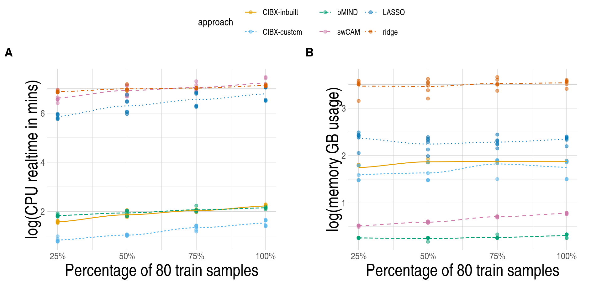
Code

## per chunk cpu time & memory for LASSO and ridge
## across 24 simulation data

expr_order[5:6]
[1] "LASSO" "RIDGE"

cluster_perchunk <- lapply(expr_order[5:6], function(appin) {
  nextflowlog[approach == appin, ][
    , {
      ncpu <- unique(cpus) %>% paste0(., collapse = "/")
      cputimes <- vtimesec(realtime) / 60
      memt <- vmem.usage(vmem) / 1024
      nchunk <- .N

      Q50c <- median(cputimes) %>% round(., 2)

      Q2575c <- quantile(cputimes, c(0.25, 0.75)) %>%
        round(., 2) %>%
        paste0(., collapse = ",")

      Q50m <- median(memt) %>% round(., 2)

      Q2575m <- quantile(memt, c(0.25, 0.75)) %>%
        round(., 2) %>%
        paste0(., collapse = ",")

      list(ncpu,
        nchunk,
        cputimes_pchunk = paste0(Q50c, " (", Q2575c, ")"),
        memt_pchunk = paste0(Q50m, " (", Q2575m, ")")
      )
    } # , by = c("simdataid", "trainper")
  ]
}) %>%
  set_names(., expr_order[5:6]) %>%
  rbindlist(., idcol = "approach")


cluster_perchunk[, approach := appro_lab[match(cluster_perchunk$approach, names(appro_lab))]]

cluster_perchunk[, approach := factor(approach, appro_lab)]


rundata_sim <- rundata4plt[,
  {
    ncpus <- unique(ncpu)
    Nsimdata <- .N
    Q50c <- median(cputimes) %>% round(., 2)
    Q2575c <- quantile(cputimes, c(0.25, 0.75)) %>%
      round(., 2) %>%
      paste0(., collapse = ",")

    Q50m <- median(memt) %>% round(., 2)
    Q2575m <- quantile(memt, c(0.25, 0.75)) %>%
      round(., 2) %>%
      paste0(., collapse = ",")

    list(ncpus,
      Ndata = Nsimdata,
      CPUmins = paste0(Q50c, " (", Q2575c, ")"),
      memGB = paste0(Q50m, " (", Q2575m, ")")
    )
  },
  by = "approach"
]


rundata_sim[cluster_perchunk, Nchunks := i.nchunk, on = "approach"]
rundata_sim[cluster_perchunk, ":="(
  cpu_perchunk = i.cputimes_pchunk,
  mem_perchunk = i.memt_pchunk
), on = "approach"]


## cpu time
sim_cputime <- rundata_sim[, tstrsplit(CPUmins, " ", keep = 1L) %>% unlist() %>% as.numeric()]
sim_cputime
[1]    7.22    3.08    7.61 1103.68  592.13 1103.60
## relative to CIBX
(sim_cputime / sim_cputime[2]) %>% round(., 2)
[1]   2.34   1.00   2.47 358.34 192.25 358.31

## mem
sim_mem <- rundata_sim[, tstrsplit(memGB, " ", keep = 1L) %>% unlist() %>% as.numeric()]
sim_mem
[1]  6.45  6.00  1.30  1.92 10.40 33.60
## relative to CIBX
(sim_mem / sim_mem[2]) %>% round(., 2)
[1] 1.07 1.00 0.22 0.32 1.73 5.60

kable(rundata_sim, caption = "resource usage metrics for the simulation data")

resource usage metrics for the simulation data
approach	ncpus	Ndata	CPUmins	memGB	Nchunks	cpu_perchunk	mem_perchunk
CIBX-inbuilt	4	24	7.22 (5.64,8.12)	6.45 (6.25,6.6)	NA	NA	NA
CIBX-custom	4	24	3.08 (2.71,4.08)	6 (4.47,6.53)	NA	NA	NA
bMIND	4	24	7.61 (6.33,8.18)	1.3 (1.3,1.3)	NA	NA	NA
swCAM	10/1	24	1103.68 (799.36,1256.04)	1.92 (1.77,2.07)	NA	NA	NA
LASSO	1	24	592.13 (391.41,862.2)	10.4 (9.46,10.94)	5377	1.88 (0.54,3.85)	10.2 (4.4,15.9)
ridge	1	24	1103.6 (1017.01,1199.88)	33.6 (32.83,35.35)	5377	4.62 (2.1,7.25)	33.1 (15.3,52.2)

2.10 SupFig10, Inbuilt and custom signature Genes, and debCAM cell type-specific genes

Code

lm22mtx_f <- file.path("CIBXres/LM22deconv", runid) %>%
  file.path(data_dir, .) %>%
  file.path(., "sigMTX4dev.txt")

cumtx_f <- file.path("CIBXres/GS", runid) %>%
  file.path(data_dir, .) %>%
  file.path(., "CIBERSORTx_refexpr4CIBXgsClass.CIBERSORTx_refexpr4CIBXgs.bm.K999.txt")
## CIBX-inbuilt and custom signature genes
sigmtx_files <- c(lm22mtx_f, cumtx_f)

## signature matrcies, inbuilt and custom,
sigmtxs <- lapply(sigmtx_files, function(filein) {
  datin <- fread(filein)
  pltmat <- datin[, -1] %>% as.matrix()
  rownames(pltmat) <- datin[[1]]

  if (ncol(pltmat) != 4) {
    ourorder <- lm22merged
    names(ourorder) <- colnames(pltmat)
    othercls <- setdiff(unique(ourorder), sctorder)
    ourorder <- sort(factor(ourorder, levels = c(sctorder, othercls)))
    pltmat <- pltmat[, names(ourorder)]
  } else {
    pltmat <- pltmat[, sctorder]
    ourorder <- NULL
  }


  min_max <- pheatmap:::scale_mat(pltmat, "row") %>% range()

  col_fun <- circlize::colorRamp2(
    seq(from = min_max[1], to = min_max[2], length.out = 11),
    cols4all::c4a("brewer.rd_bu", n = 11, reverse = TRUE)
  )

  list(
    pltmat = pltmat,
    col_fun = col_fun,
    matorder = ourorder
  )
})

names(sigmtxs) <- c("inbuilt", "custom")

figS10ab <- lapply(sigmtxs, "[[", "pltmat")
names(figS10ab) <- paste0("figS10", letters[seq_along(figS10ab)])


## Lm22 merged text
ourorder <- sigmtxs$inbuilt$matorder
descri.text <- NULL
for (cttype in unique(ourorder)) {
  descri.text <- c(
    descri.text,
    sprintf(
      "%s: %s",
      cttype,
      names(ourorder)[ourorder == cttype] %>% combine_words()
    )
  )
}

descri.text
 [1] "CD4: T cells CD4 naive, T cells CD4 memory resting, T cells CD4 memory activated, T cells follicular helper, and T cells regulatory (Tregs)"
 [2] "CD8: T cells CD8"                                                                                                                           
 [3] "CD14: Monocytes, Macrophages M0, Macrophages M1, and Macrophages M2"                                                                        
 [4] "CD19: B cells naive and B cells memory"                                                                                                     
 [5] "PCs: Plasma cells"                                                                                                                          
 [6] "GammaT: T cells gamma delta"                                                                                                                
 [7] "NK: NK cells resting and NK cells activated"                                                                                                
 [8] "Dendritic: Dendritic cells resting and Dendritic cells activated"                                                                           
 [9] "Mast: Mast cells resting and Mast cells activated"                                                                                          
[10] "Eos: Eosinophils"                                                                                                                           
[11] "PMN: Neutrophils"                                                                                                                           

gpar(fontface = "bold")
$font
bold 
   2 
## https://github.com/wilkelab/gridtext/issues/24
update_gpar <- function(gp, gp_new) {
  names_new <- names(gp_new)
  names_old <- names(gp)
  gp[c(intersect(names_old, names_new), "fontface")] <- NULL
  gp_new["fontface"] <- NULL
  do.call(gpar, c(gp, gp_new))
}
gp <- gpar(fontface = "bold")
gpmod <- update_gpar(gp, gpar(fontsize = 10))


## heatmaps for inbuilt and custom
ht_sigmtx <- lapply(names(sigmtxs), function(nin) {
  datmtx <- sigmtxs[[nin]]$pltmat %>%
    pheatmap:::scale_mat(., "row")
  datcol <- sigmtxs[[nin]]$col_fun
  datsplit <- sigmtxs[[nin]]$matorder

  Heatmap(
    matrix = datmtx, col = datcol,
    cluster_columns = FALSE,
    show_row_names = FALSE,
    column_split = datsplit,
    column_gap = unit(1, "mm"),
    ## column_title_gp = gpar(fontface = "bold",
    ##                        fontsize=10),
    column_title_gp = gpmod,
    name = paste0(nin, "\nExpr")
  )
})

names(ht_sigmtx) <- names(sigmtxs)

Code

## observed expr
observ_expr <- file.path(
  data_dir,
  "CLUSTERData/ObservTPMExpr.rds"
) %>%
  readRDS()

########################################################
## sig genes in observ_expr, including debCAM markers ##
########################################################

## cell type train and testing samples
sampin4pca <- sampdata[celltype != "PBMC" & samtype == "nonrefsamp", sample]
## sampin4pca <- sampdata[celltype!="PBMC", sample]

pca1_4res <- list(
  inbuilt = rownames(sigmtxs$inbuilt$pltmat),
  custom = rownames(sigmtxs$custom$pltmat),
  debCAM = unlist(debCAMresFract$OVE.FC_10$markers, use.names = FALSE)
) %>% lapply(., function(sgin) {
  ## some LM22 genes are not found in observ_expr
  gin <- intersect(sgin, rownames(observ_expr))

  ## pca of signature genes in our observed expr
  mat <- log2(observ_expr[gin, sampin4pca] + 1)
  mat %>% dim()

  pca_res <- prcomp(t(mat))

  pcs <- pca_res$x[, seq(1, 4)] %>% as.data.frame()
  pcs$celltype <- sampdata$celltype[match(rownames(pcs), sampdata$sample)]
  pcs$celltype <- factor(pcs$celltype, levels = sctorder)
  pcs$Batch <- sampdata$batch[match(rownames(pcs), sampdata$sample)]
  pcs$Batch <- factor(pcs$Batch)

  pcaplts <- lapply(1:2, function(x) {
    x1 <- paste0("PC", 2 * x - 1)
    y1 <- paste0("PC", 2 * x)
    ggscatter(pcs,
      x = x1, y = y1,
      fill = "celltype",
      shape = "Batch",
      alpha = 0.9,
      ellipse = TRUE,
      ellipse.type = "convex",
      ellipse.alpha = 0.3,
      ellipse.border.remove = TRUE,
      palette = ctfrat.pal
    ) +
      scale_shape_manual(
        values = c(
          "1" = 21,
          "2" = 22,
          "3" = 23,
          "4" = 24
        ),
        limits = force
      ) +

      guides(fill = guide_legend(override.aes = list(shape = 21))) +

      used_ggthemes()
  }) %>% ggarrange(plotlist = ., common.legend = TRUE)

  list(
    gin = gin,
    pcaplts = pcaplts
  )
})


figS10def <- list(
  inbuilt = rownames(sigmtxs$inbuilt$pltmat),
  custom = rownames(sigmtxs$custom$pltmat),
  debCAM = unlist(debCAMresFract$OVE.FC_10$markers, use.names = FALSE)
) %>% lapply(., function(sgin) {
  ## some LM22 genes are not found in observ_expr
  gin <- intersect(sgin, rownames(observ_expr))

  ## pca of signature genes in our observed expr
  mat <- log2(observ_expr[gin, sampin4pca] + 1)
  mat %>% dim()

  pca_res <- prcomp(t(mat))

  pcs <- pca_res$x[, seq(1, 4)] %>% as.data.frame()
  pcs$celltype <- sampdata$celltype[match(rownames(pcs), sampdata$sample)]
  pcs$celltype <- factor(pcs$celltype, levels = sctorder)
  pcs$Batch <- sampdata$batch[match(rownames(pcs), sampdata$sample)]
  pcs$Batch <- factor(pcs$Batch)
  pcs
})


names(figS10def) <- paste0("figS10", c("d", "e", "f"))

Expression of inbuilt signature genes (N=547) in 22 leukocyte subsets, curated by the CIBERSORTx team from microarray gene expression. For each gene (row), expression is centred to the mean and scaled by the standard deviation of cell types (column). Columns are split by the collapsed classes. CD4: T cells CD4 naive, T cells CD4 memory resting, T cells CD4 memory activated, T cells follicular helper, and T cells regulatory (Tregs); CD8: T cells CD8; CD14: Monocytes, Macrophages M0, Macrophages M1, and Macrophages M2; CD19: B cells naive and B cells memory; PCs: Plasma cells; GammaT: T cells gamma delta; NK: NK cells resting and NK cells activated; Dendritic: Dendritic cells resting and Dendritic cells activated; Mast: Mast cells resting and Mast cells activated; Eos: EosinophilsPMN: Neutrophils

Code

## inbuilt signature genes
ht_sigmtx[[1]]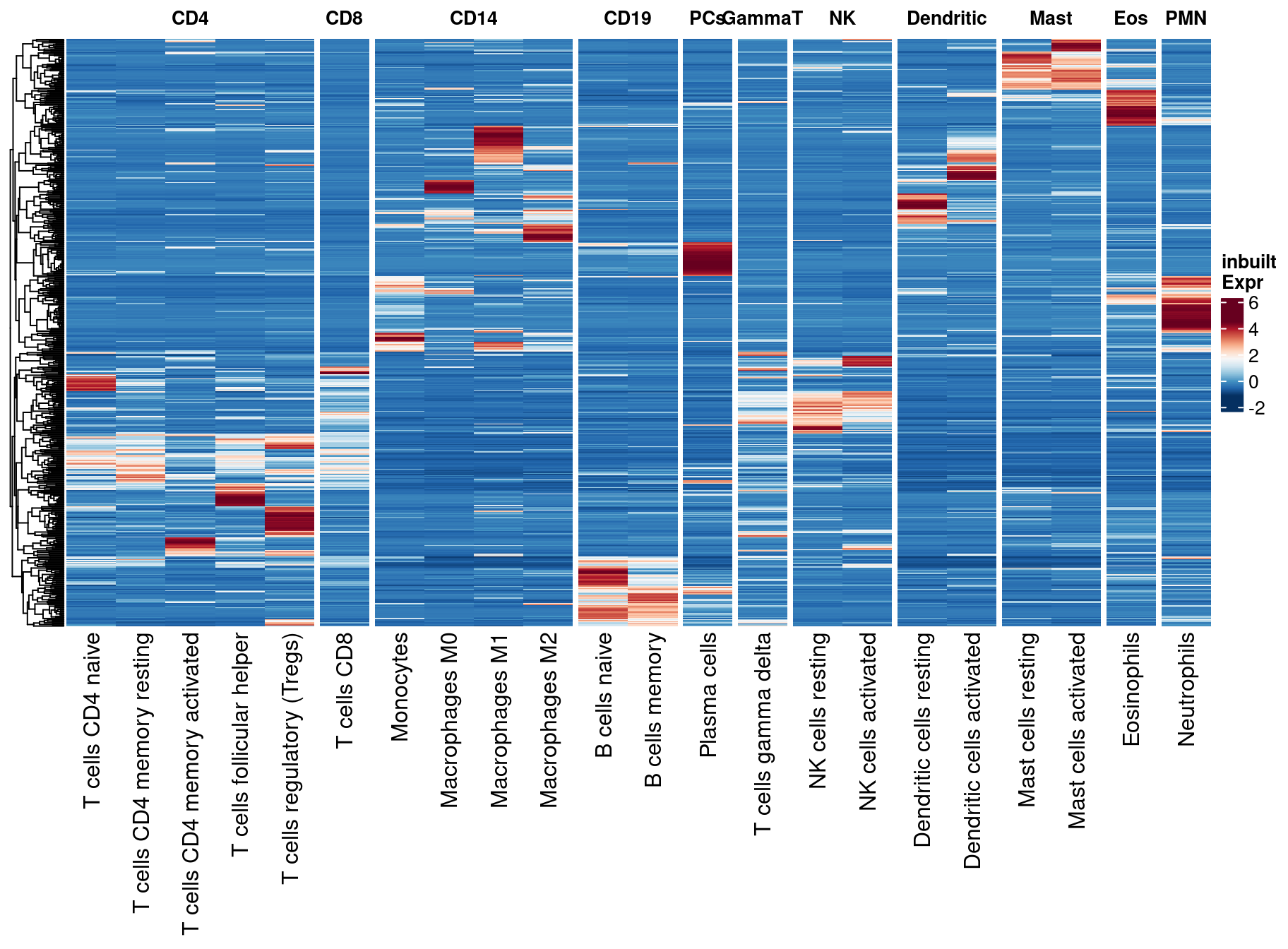

Expression of custom signature genes (N=1589), derived from our sorted-cell RNAseq expression in 80 training subjects using CIBERSORTx. Expression is centred and scaled across cell types (column) by gene (row).

Code

## custom signature genes

ht_sigmtx[[2]]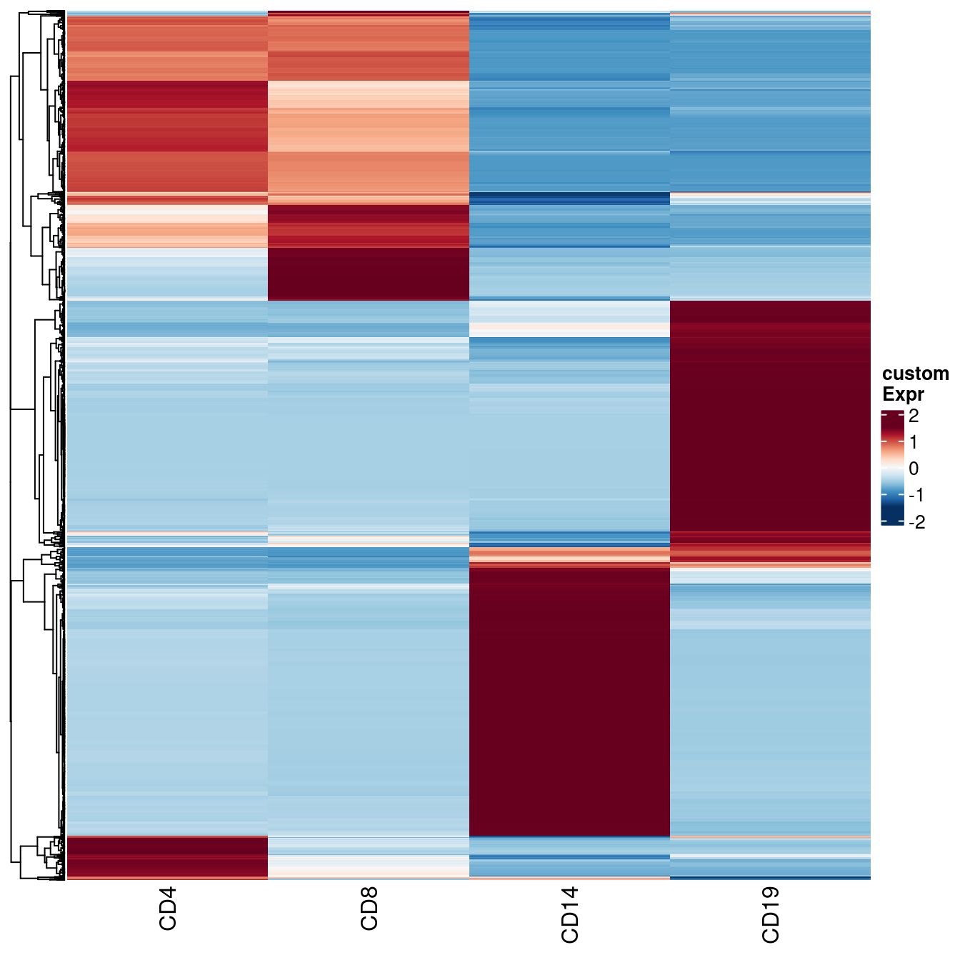

Numbers (No.) of debCAM cell-type specific genes by cell type (row) and selection criteria (column). debCAM, which does not have the signature matrix, selects the cell-type-specific genes, that are over-expressed (OVE) in one cell type compared to others combined. OVE fold change (FC) of 1, 2, 5 and 10 were used in debCAM on our sorted cell expression in 80 training subjects.

Code

## debCAM cell type-specific genes by fold changes
## supple for debCAM
## summary of no. markers by 4 FCs

debCAMmarkers <- lapply(debCAMresFract, function(dat) {
  sapply(dat$markers, function(x) {
    length(x)
  })
}) %>%
  do.call(rbind, .) %>%
  as.data.frame() %>%
  setDT(., keep.rownames = TRUE)

## no. markers by fc from debcam
debbarplt <- melt(debCAMmarkers, id.vars = "rn", measure.vars = sctorder, variable.name = "celltype", variable.factor = sctorder)[, rn := factor(rn, names(debCAMresFract))] %>%
  ggplot(data = ., aes(x = celltype, y = value)) +
  geom_bar(stat = "identity", fill = "#69b3a2", width = 0.8) +
  geom_text(aes(label = value, hjust = ifelse(value < 500, 0, 0.8)), size = 3.5) +
  coord_flip() +
  facet_wrap(~rn, ncol = 4) +
  ylab("No. cell-type specific genes") +
  xlab("cell type") +
  used_ggthemes()


debbarplt

figS10c <- melt(debCAMmarkers, id.vars = "rn", measure.vars = sctorder, variable.name = "celltype", variable.factor = sctorder)[, rn := factor(rn, names(debCAMresFract))]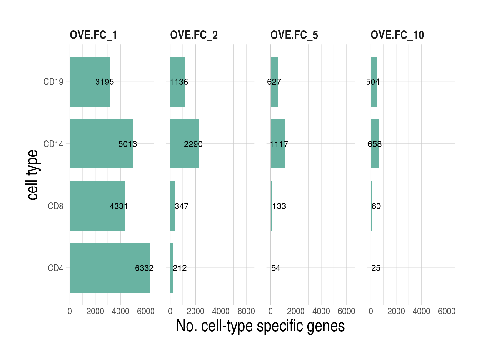

The first four principal components from PCA analysis of inbuilt signature gene expression in test samples. Each dot is a sample, coloured by cell type and shaped by sequencing batch.

Code

## PCA analysis of cell type expression data in test samples
### inbuilt signature genes

pca1_4res$inbuilt$pcaplts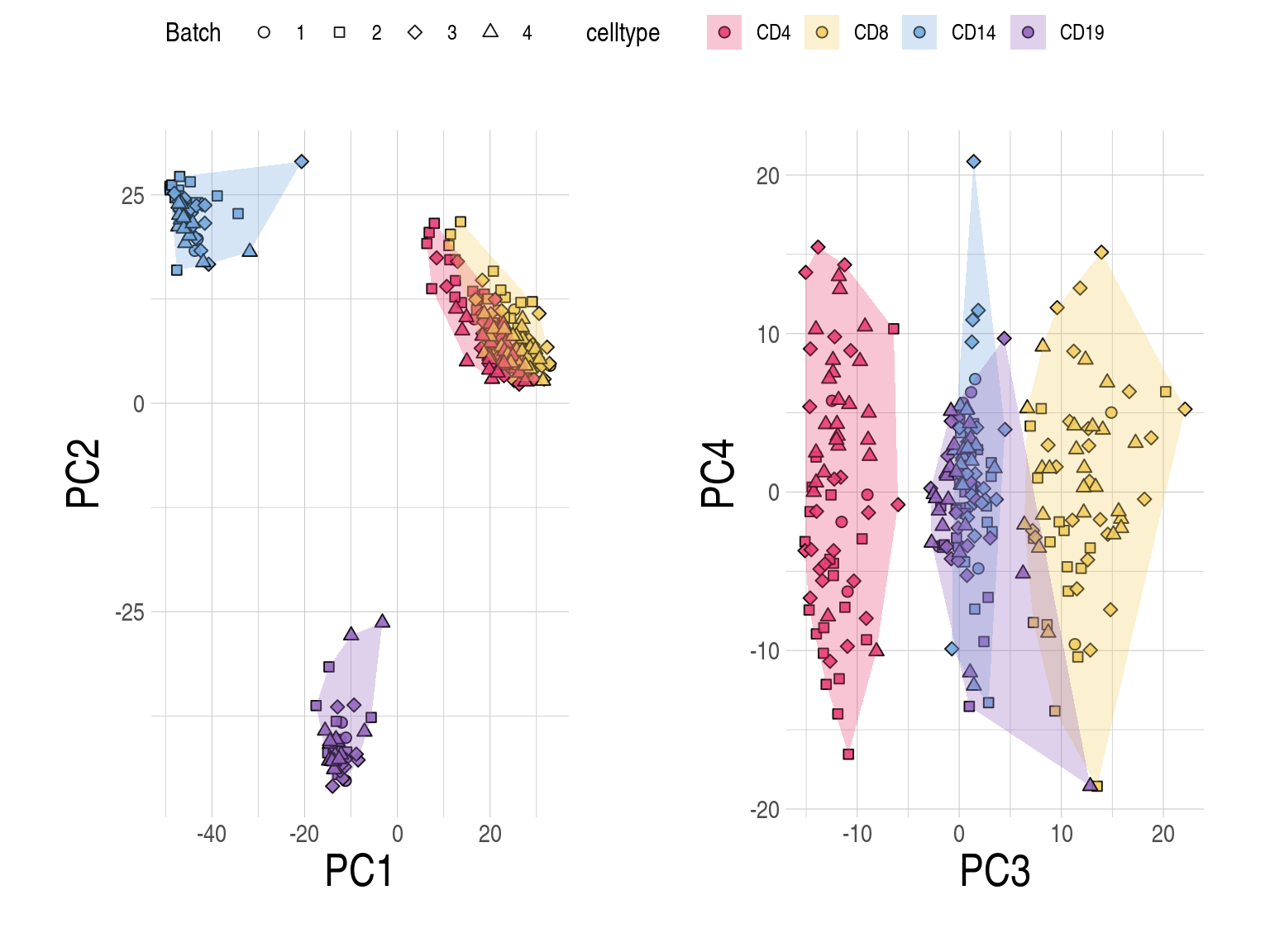

The first four principal components from PCA analysis of custom signature gene expression in test samples.

Code

### custum signature genes
pca1_4res$custom$pcaplts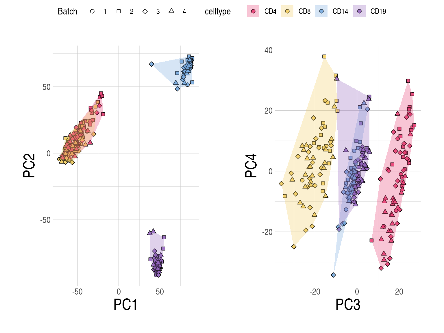

The first four principal components from PCA analysis of debCAM cell-type specific gene expression in test samples.

Code

### debCAM cell-type specific genes

pca1_4res$debCAM$pcaplts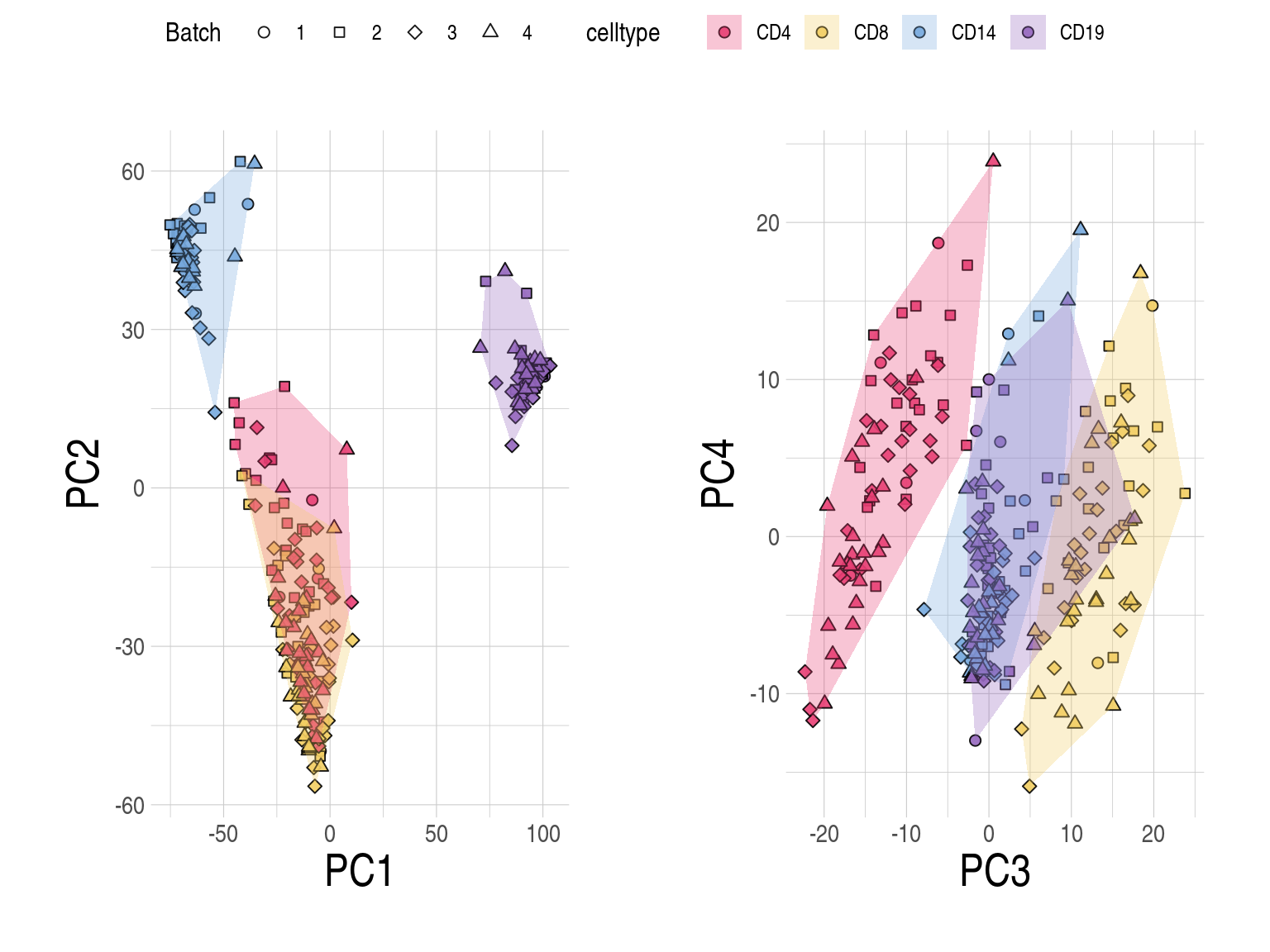

2.11 SupFig12, Combat-seq

The first four principal components from PCA analysis of log2(count-per-million) expression derived from raw read counts in RNAseq samples used in this work.

Code

res_d <- file.path(data_dir, "ZenodoCLUSTER")
rawreadtbl <- read.table(file.path(res_d, "RawReadCounts_Zenodo.csv"), row.names = 1, sep = ",", header = TRUE)
rawreadtbl <- rawreadtbl[, sampdata$sample]

adjreadtbl <- file.path(res_d, "BatchCorrectedReadCounts_Zenodo.csv") %>%
  read.table(file = ., row.names = 1, sep = ",", header = TRUE)
adjreadtbl <- adjreadtbl[, sampdata$sample]

geneMeta <- file.path(res_d, "GeneMetaInfo_Zenodo.csv") %>%
  read.table(
    file = ., row.names = 1, sep = ",",
    header = TRUE
  )


pca_res <- list(rawreadtbl, adjreadtbl) %>%
  lapply(., function(countmtx) {
    objinput <- DGEList(
      counts = countmtx,
      genes = geneMeta[match(rownames(countmtx), geneMeta$Geneid), ]
    )

    keep <- filterByExpr(objinput,
      group = sampdata$celltype[match(colnames(objinput), sampdata$sample)]
    )
    objinput <- objinput[keep, , keep.lib.sizes = FALSE]
    objinput <- calcNormFactors(objinput)
    matcpm <- cpm(objinput, log = TRUE)
    respca <- prcomp(x = t(matcpm))
    stopifnot(all(rownames(respca$x) == sampdata$sample))
    dsn4pca <- cbind(respca$x[, 1:4], sampdata[, .(celltype, batch)])
    dsn4pca$batch <- factor(dsn4pca$batch, levels = 1:4)
    dsn4pca$celltype <- factor(
      dsn4pca$celltype,
      levels = c("PBMC", sctorder)
    )
    dsn4pca
  })


figS12ab <- copy(pca_res)
names(figS12ab) <- paste0("figS12", letters[seq_along(pca_res)])

ctfrat.palpmbc <- c(ctfrat.pal, "#AAAA00")
names(ctfrat.palpmbc) <- c(sctorder, "PBMC")

pca_plts <- lapply(pca_res, function(datin) {
  pcaplts <- lapply(1:2, function(x) {
    x1 <- paste0("PC", 2 * x - 1)
    y1 <- paste0("PC", 2 * x)

    ggscatter(datin,
      x = x1, y = y1,
      fill = "celltype",
      shape = "batch",
      alpha = 0.9,
      palette = ctfrat.palpmbc
    ) +
      scale_shape_manual(
        values = c(
          "1" = 21,
          "2" = 22,
          "3" = 23,
          "4" = 24
        ),
        limits = force
      ) +
      guides(fill = guide_legend(override.aes = list(shape = 21))) +
      used_ggthemes()
  })
})

## raw
ggarrange(plotlist = pca_plts[[1]], common.legend = TRUE)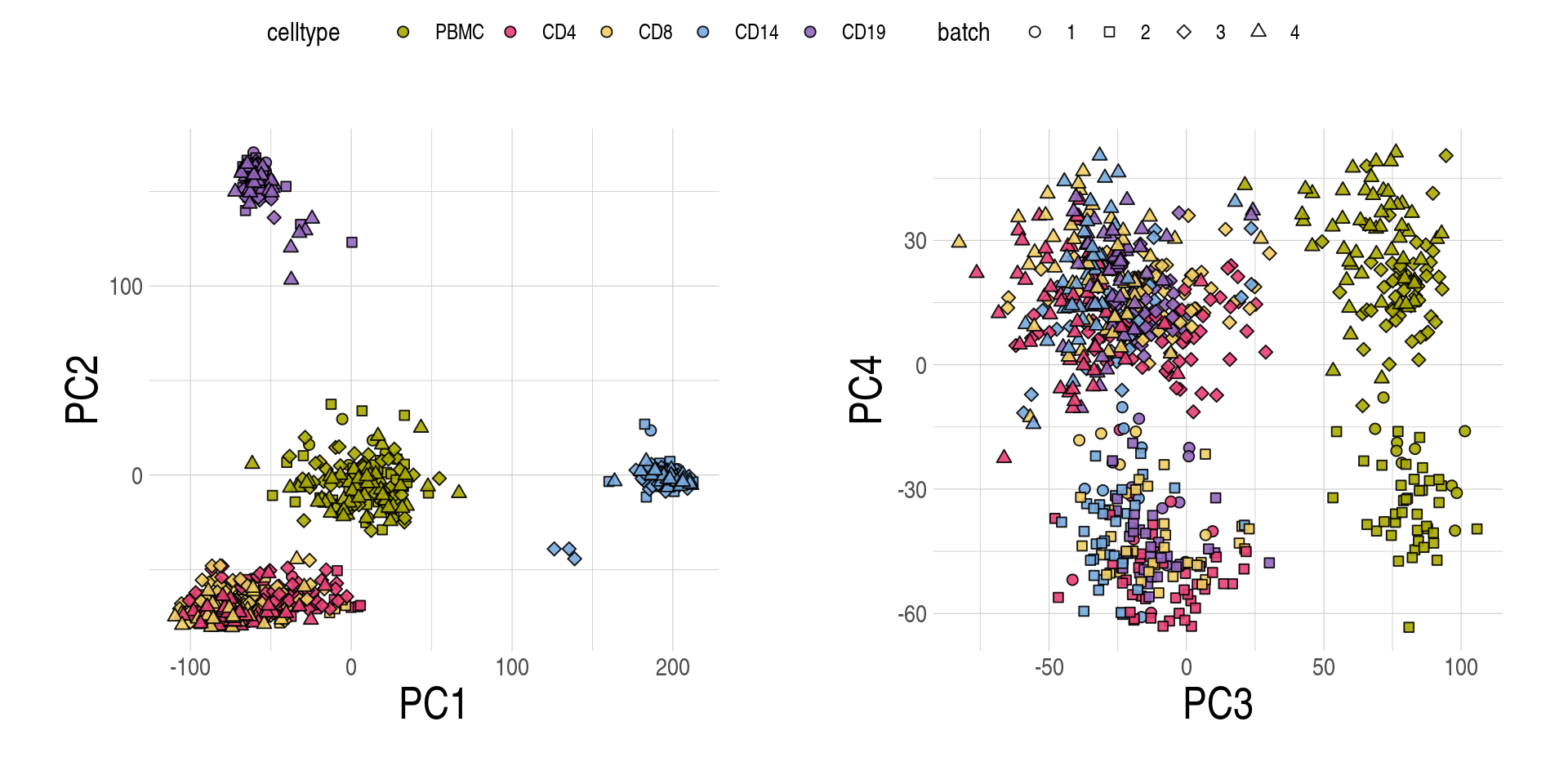

The first four principal components from PCA analysis of log2(count-per-million) expression derived from Combat-Seq batch-adjusted read counts in RNAseq samples used in this work

Code

## combat-seq

ggarrange(plotlist = pca_plts[[2]], common.legend = TRUE)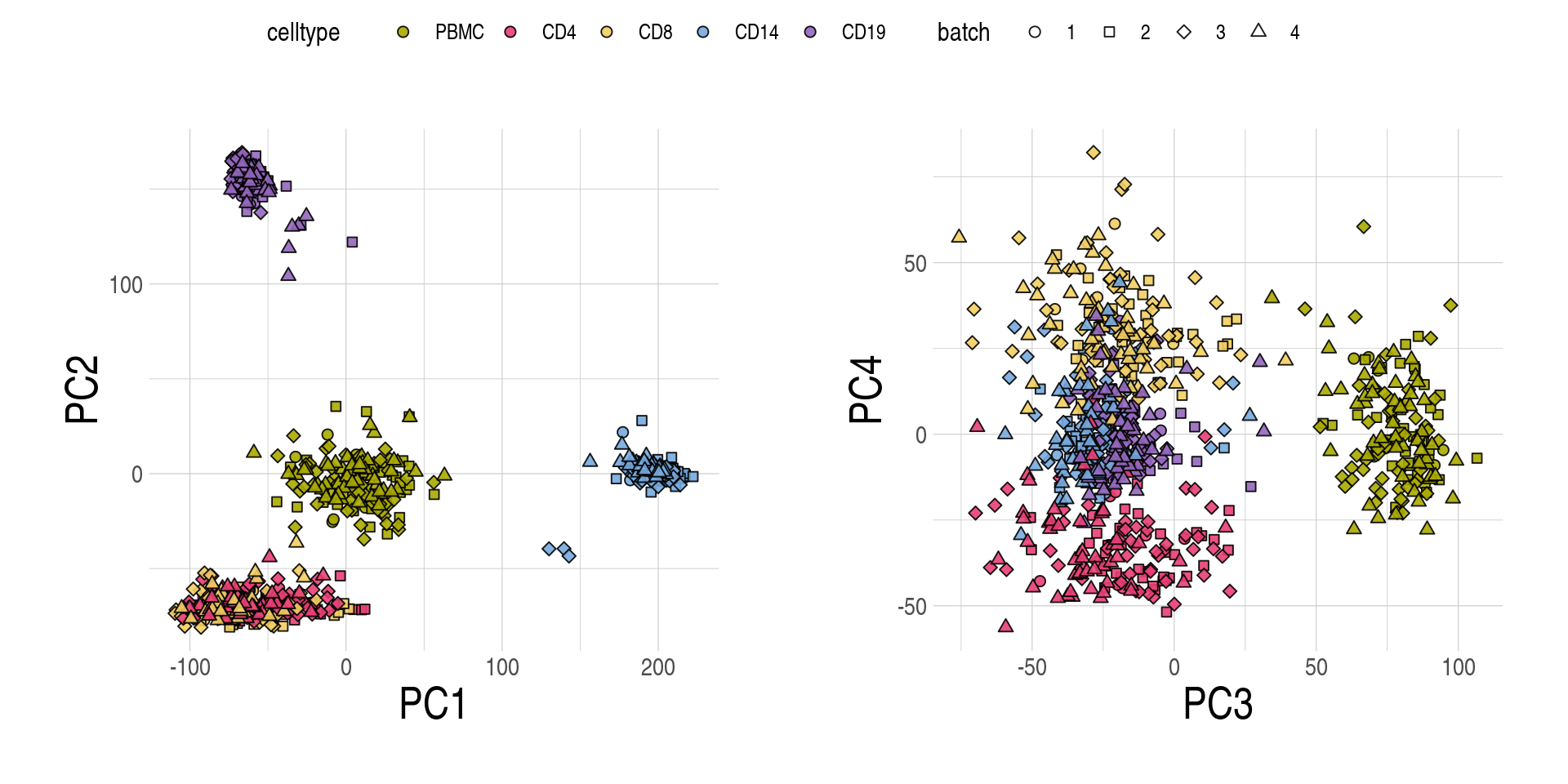

2.12 SupFig13, Batch composition of subjects by train and test set

Frequencies (A) and percentages (B) of subjects by batch and training/testing set.

Code

## Batch composition of subjects by train and test set
categoryplt <- function(dat, xgroup, fillvar, ...) {
  ## count
  adsn <- dat[!is.na(get(xgroup)), .N, by = c(xgroup, fillvar)][eval(parse(text = paste0("order(", xgroup, ",", fillvar, ")")))]

  ares <- adsn %>% ggbarplot(
    data = ., x = xgroup, y = "N",
    fill = fillvar,
    ylab = "Counts", ...
  )
  ## percentage
  bdsn <- dat[!is.na(get(xgroup)), .N, by = c(xgroup, fillvar)][eval(parse(text = paste0("order(", xgroup, ",", fillvar, ")")))]
  bdsn <- bdsn[,
    {
      an <- sum(N)
      props <- N / an
      labelt <- round(props, 2)
      list(eval(parse(text = fillvar)), N, an, props, labelt)
    },
    by = xgroup
  ]

  bres <- bdsn %>% ggbarplot(
    data = ., x = xgroup, y = "labelt", fill = "V1",
    ylab = "Percentages", ...
  )
  bres

  overp <- chisq.test(dat[[fillvar]], dat[[xgroup]])$p.value
  overp <- ifelse(overp < 10^-2,
    paste0("=", format(overp,
      nsmall = 2,
      digits = 3,
      scientific = TRUE
    )),
    paste0("=", round(overp, 2))
  )
  if (class(dat[[xgroup]]) == "character") {
    dat[[xgroup]] <- factor(dat[[xgroup]])
  }
  ## grp <- unique(dat[[xgroup]])
  grp <- levels(dat[[xgroup]])
  dddf <- data.table(
    group1 = grp[1], group2 = grp[length(grp)],
    p = paste0(" p ", overp)
  )
  bres <- bres +
    stat_pvalue_manual(dddf,
      y.position = 1.02,
      bracket.nudge.y = 0.02,
      label = "Chi-square test, {p}"
    ) +
    labs(fill = fillvar)

  list(ares, bres)
}

## subjects by train and test set
sampdata.sub <- unique(sampdata, by = "samp")
sampdata.sub[, Batch := factor(batch, levels = seq(1, 4))]
sampdata.sub[, sample_type := factor(samtype, levels = c("refsamp", "nonrefsamp"), labels = c("train", "Test"))]

categoryplt(
  dat = sampdata.sub,
  xgroup = "sample_type",
  fillvar = "Batch",
  xlab = FALSE,
  label = TRUE,
  lab.pos = "in",
  palette = "jama"
) %>%
  ggarrange(plotlist = ., common.legend = TRUE, labels = LETTERS)

figS13 <- sampdata.sub[, .(samp, sample_type, Batch)]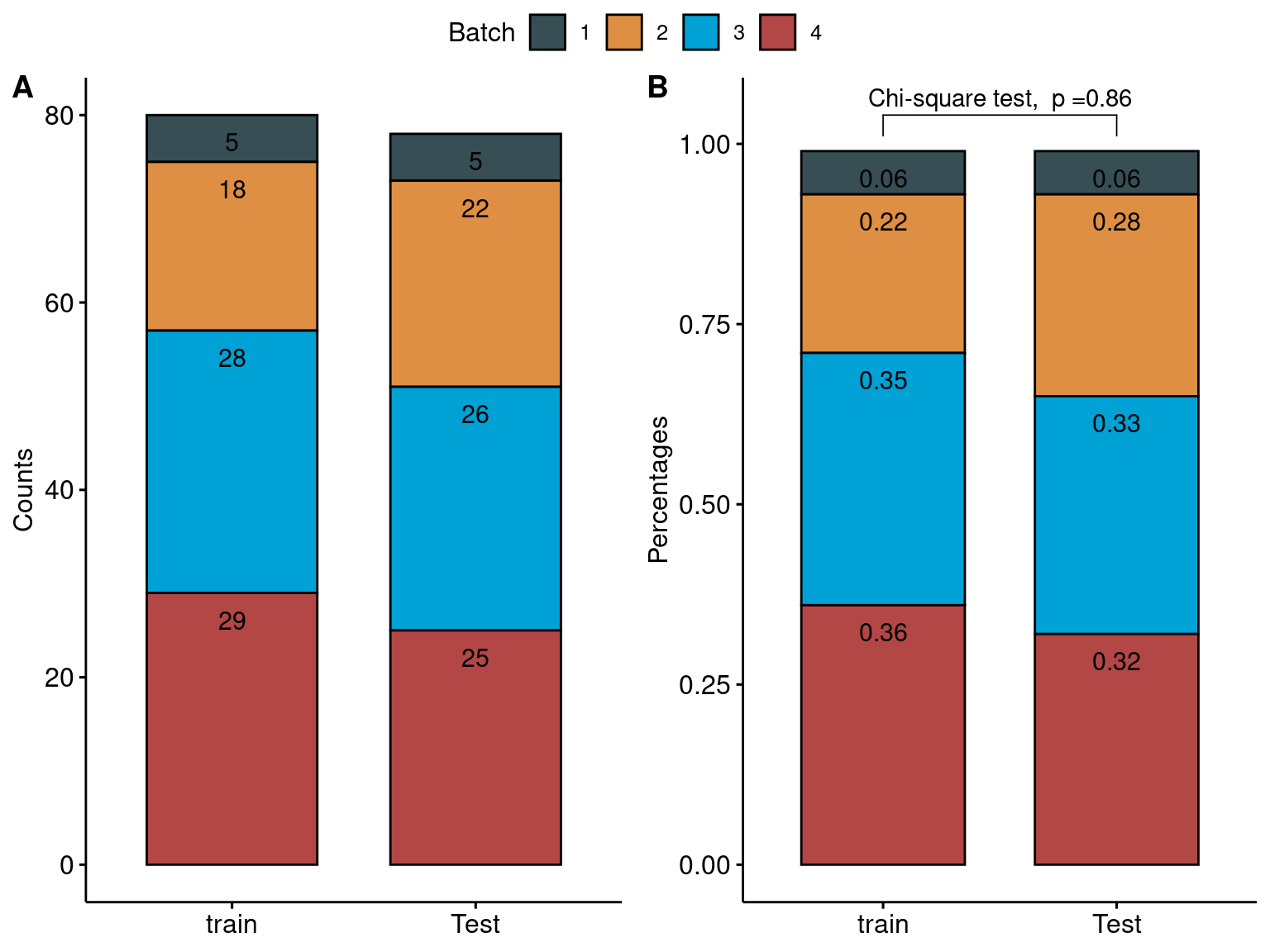

2.13 SupFig14, Correalations of fractions between inbuilt cell linages with true flow data

Code

## Fractions between 22 inbuilt cell lineages with flow data
####################
## flow fractions ##
####################
fractflow <- file.path(data_dir, "CLUSTERData/flowFract_wide.rds") %>%
  readRDS() %>%
  as.matrix()

## cibx-LM22
#############################
## fractions based on LM22 ##
#############################
lm22merged <- "data4repo/mergedClasses.csv" %>%
  file.path(here::here(), .) %>%
  scan(., what = "character", sep = "\t")

lm22mtx <- lm22mtx_f %>% fread()

res_d <- file.path("CIBXres/LM22deconv", runid) %>%
  file.path(data_dir, .)
res_d
[1] "/rds/project/rds-csoP2nj6Y6Y/wyl37/Rbookdown/sceQTLGen/CLUSTERdeconRes/CIBXres/LM22deconv/cluster"

lm22res <- file.path(res_d, "CIBERSORTxGEP_NA_Fractions-Adjusted.txt") %>%
  fread()

stopifnot(names(lm22res)[-1][1:length(names(lm22mtx)[-1])] == names(lm22mtx)[-1])

## fractions in 22 cell types
lm22res.mtx <- lm22res[, names(lm22mtx)[-1], with = FALSE] %>% as.matrix()
rownames(lm22res.mtx) <- lm22res$Mixture

ourorder <- lm22merged
names(ourorder) <- names(lm22mtx)[-1]
othercls <- setdiff(unique(ourorder), sctorder)
ourorder <- sort(factor(ourorder, levels = c(sctorder, othercls)))

## sample order matched to fractflow
lm22res.mtx <- lm22res.mtx[rownames(fractflow), names(ourorder)]

## test samples
nonrefsamps <- sampdata[samtype == "nonrefsamp" & celltype == "PBMC", sample]

## correlation
mychks_test <- cor(
  x = fractflow[nonrefsamps, ],
  y = lm22res.mtx[nonrefsamps, ]
)

annotcoldf <- data.frame(mergedClass = ourorder)
rownames(annotcoldf) <- names(ourorder)

## find column split
kkkres <- S4Vectors::Rle(ourorder)


annotcol_pal <- friend11
names(annotcol_pal) <- levels(ourorder)

annotcol_pal_dat <- list(mergedClass = annotcol_pal)


## heatmap correlation
library(circlize)
col_fun <- circlize::colorRamp2(
  c(1, 0, -1),
  colorspace::diverging_hcl(palette = "Red-Green", n = 3)
)

gp <- gpar(fontface = "bold")
update_gpar(gp, gpar(fontsize = 10))
$font
[1] 2

$fontsize
[1] 10

beforeCorht <- ComplexHeatmap::pheatmap(
  mat = mychks_test,
  name = "Cor",
  color = col_fun,
  cluster_rows = FALSE, cluster_cols = FALSE,
  display_numbers = TRUE, number_format = "%.2f",
  number_color = "black",
  annotation_col = annotcoldf,
  annotation_colors = annotcol_pal_dat,
  gaps_col = S4Vectors::end(kkkres),
  cellwidth = 25, cellheight = 25,
  row_names_side = "left"
)

figS14 <- mychks_test

Pearson correlations between inbuilt LM22 and ground-truth flow fractions. Columns are LM22 cell subsets split by their merged classes (top annotation). Rows are ground truth cell types. Each cell is coloured based on the strength of the correlation.

Code

beforeCorht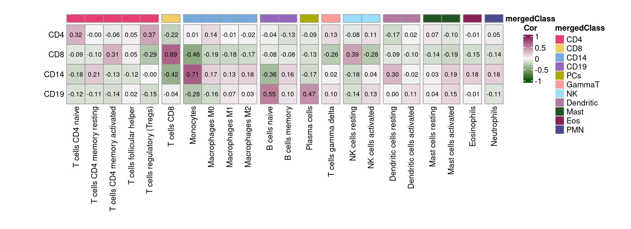

Code

ddd <- ls(pattern = "figS") %>% str_sort(., numeric = TRUE)
dddidx <- sapply(ddd, get) %>% sapply(., function(x) inherits(x, "list"))

cccin <- ddd[!dddidx]
ccc <- vector(mode = "list", length = length(cccin))
for (i in seq_along(cccin)) {
  ccc[[i]] <- get(cccin[i])
}
names(ccc) <- cccin

ddd[dddidx]
[1] "figS1"     "figS10ab"  "figS10def" "figS12ab" 

outlist <- c(
  figS1, ccc[1:12],
  figS10ab, ccc["figS10c"],
  figS12ab, ccc[14:15]
)

names(outlist) <- toupper(names(outlist)) %>%
  str_extract(., pattern = "S.+$") %>%
  paste0(., "_fig")

openxlsx::write.xlsx(outlist,
  file = "SourceData_SuppFigures.xlsx"
)

2.14 AUCs in Test samples, CLUSTER data

Code

rds_f <- "fig4rundatatestonly.rds"

if (!file.exists(rds_f)) {
  ## main: different gene set; common: same genes per cell across methods
  ## impvexpr_all <- list(main = expr_ori, common = expr_scenarios)
  impvexpr_all <- list(
    main = cdata_explst$iexpr,
    common = cdata_explst$icexpr
  )

  ## TRUE for dichotomous; FALSE for continuous
  dcht_pheno <- c(TRUE, FALSE)
  names(dcht_pheno) <- c("dcht", "cntn")

  numCores <- length(expr_order)
  numCores

  cl <- makeCluster(numCores, type = "FORK")
  registerDoParallel(cl)

  aucall <- foreach(
    j = seq_along(impvexpr_all),
    .final = function(x) setNames(x, names(impvexpr_all))
  ) %:%
    foreach(
      i = dcht_pheno,
      .final = function(x) setNames(x, names(dcht_pheno))
    ) %dopar% {
      observy <- cdata_explst$oexpr
      train_samps_ct <- cdata_explst$trainsamp
      sampdata <- cdata_explst$phenodata

      dat <- run_datprepfig4(
        obvexpr = observy,
        impvexpr = impvexpr_all[[j]],
        tsampct = NULL,
        dich = i
      )
      ## expr ~ pheno
      res1 <- run_fig4(datprlst = dat, truesig = 0.05)

      ## expr~ sex + pheno
      res2 <- run_fig4(
        datprlst = dat, truesig = 0.05,
        covdata = sampdata, covid = "sample", covar = "sex"
      )

      list(nocov = res1, covin = res2)
    }

  stopCluster(cl)

  mychktestonly <- unlist(aucall, recursive = FALSE) %>%
    unlist(., recursive = FALSE) %>%
    lapply(., "[[", "aucres") %>%
    lapply(., function(datin) {
      datin[, ":="(
        celltype = factor(celltype, levels = sctorder),
        approach = factor(approach, levels = expr_order))]
      datin
    }) %>%
    rbindlist(l = ., idcol = "scenarios") %>%
    .[, pheno := gsub("^main\\.|^common\\.", "", scenarios)] %>%
    .[, scenario := str_extract(scenarios, "main|common")]

  saveRDS(mychktestonly, file = rds_f)
} else {
  mychktestonly <- readRDS(rds_f)
}

2.14.1 Varying gene sets

Code

pheno.order <- CJ(c("dcht", "cntn"), c("nocov", "covin"), sorted = FALSE)[, paste(V1, V2, sep = ".")]
pheno.order
[1] "dcht.nocov" "dcht.covin" "cntn.nocov" "cntn.covin"
mychktestonly[, pheno := factor(pheno, levels = pheno.order, labels = c("dichPheno", "dichPheno+sex", "contPheno", "contPheno+sex"))]

## no. auc available
achk <- mychktestonly[scenario == "main" & !is.na(auc), .N, by = c("pheno", "celltype", "approach")][N != 10, ]
achk
            pheno celltype approach N
 1:     dichPheno      CD8  inbuilt 8
 2:     dichPheno      CD8   custom 8
 3:     dichPheno      CD8    bMIND 9
 4:     dichPheno      CD8    swCAM 9
 5:     dichPheno      CD8    LASSO 9
 6:     dichPheno      CD8    RIDGE 9
 7:     dichPheno     CD14  inbuilt 7
 8:     dichPheno     CD14   custom 8
 9:     dichPheno     CD14    bMIND 7
10:     dichPheno     CD14    swCAM 7
11:     dichPheno     CD14    LASSO 7
12:     dichPheno     CD14    RIDGE 7
13:     dichPheno     CD19  inbuilt 8
14:     dichPheno     CD19   custom 8
15:     dichPheno     CD19    bMIND 8
16:     dichPheno     CD19    swCAM 8
17:     dichPheno     CD19    LASSO 8
18:     dichPheno     CD19    RIDGE 8
19: dichPheno+sex      CD4  inbuilt 9
20: dichPheno+sex      CD4   custom 8
21: dichPheno+sex      CD8  inbuilt 7
22: dichPheno+sex      CD8   custom 7
23: dichPheno+sex      CD8    bMIND 8
24: dichPheno+sex      CD8    swCAM 8
25: dichPheno+sex      CD8    LASSO 8
26: dichPheno+sex      CD8    RIDGE 8
27: dichPheno+sex     CD14  inbuilt 8
28: dichPheno+sex     CD14   custom 8
29: dichPheno+sex     CD14    bMIND 7
30: dichPheno+sex     CD14    swCAM 7
31: dichPheno+sex     CD14    LASSO 7
32: dichPheno+sex     CD14    RIDGE 7
33: dichPheno+sex     CD19  inbuilt 8
34: dichPheno+sex     CD19   custom 8
35: dichPheno+sex     CD19    bMIND 9
36: dichPheno+sex     CD19    swCAM 9
37: dichPheno+sex     CD19    LASSO 9
38: dichPheno+sex     CD19    RIDGE 9
39:     contPheno      CD8  inbuilt 9
40:     contPheno     CD14  inbuilt 9
41:     contPheno     CD14   custom 9
42:     contPheno     CD14    bMIND 9
43:     contPheno     CD14    swCAM 9
44:     contPheno     CD14    LASSO 8
45:     contPheno     CD14    RIDGE 9
46: contPheno+sex     CD14  inbuilt 9
47: contPheno+sex     CD14   custom 9
48: contPheno+sex     CD14    LASSO 9
49: contPheno+sex     CD19  inbuilt 9
            pheno celltype approach N

achk_words <- "**Noted AUC was not calculated for some simulated phenotypes because all associations were true negative, and none were false negative. Scenario-celltype-approach with no. AUCs $<$ 10 are listed in the code chunk.**"


ggboxplot(
  data = mychktestonly[scenario == "main", ],
  x = "approach", y = "auc", ylab = "AUC",
  palette = appro.cols,
  alpha = 0.35, fill = "approach",
  add = c("jitter"),
  add.params = list(shape = 21, size = 2.5, alpha = 1)
) +
  scale_fill_manual(labels = appro_lab, values = appro.cols) +
  facet_grid(pheno ~ celltype, scales = "free") +
  labs(fill = NULL) +
  used_ggthemes(
    axis.text.x = element_blank(),
    legend.position = "top",
    strip.text.y.right = element_text(angle = 0),
    legend.text = element_text(size = rel(1))
  ) +
  rremove("xlab")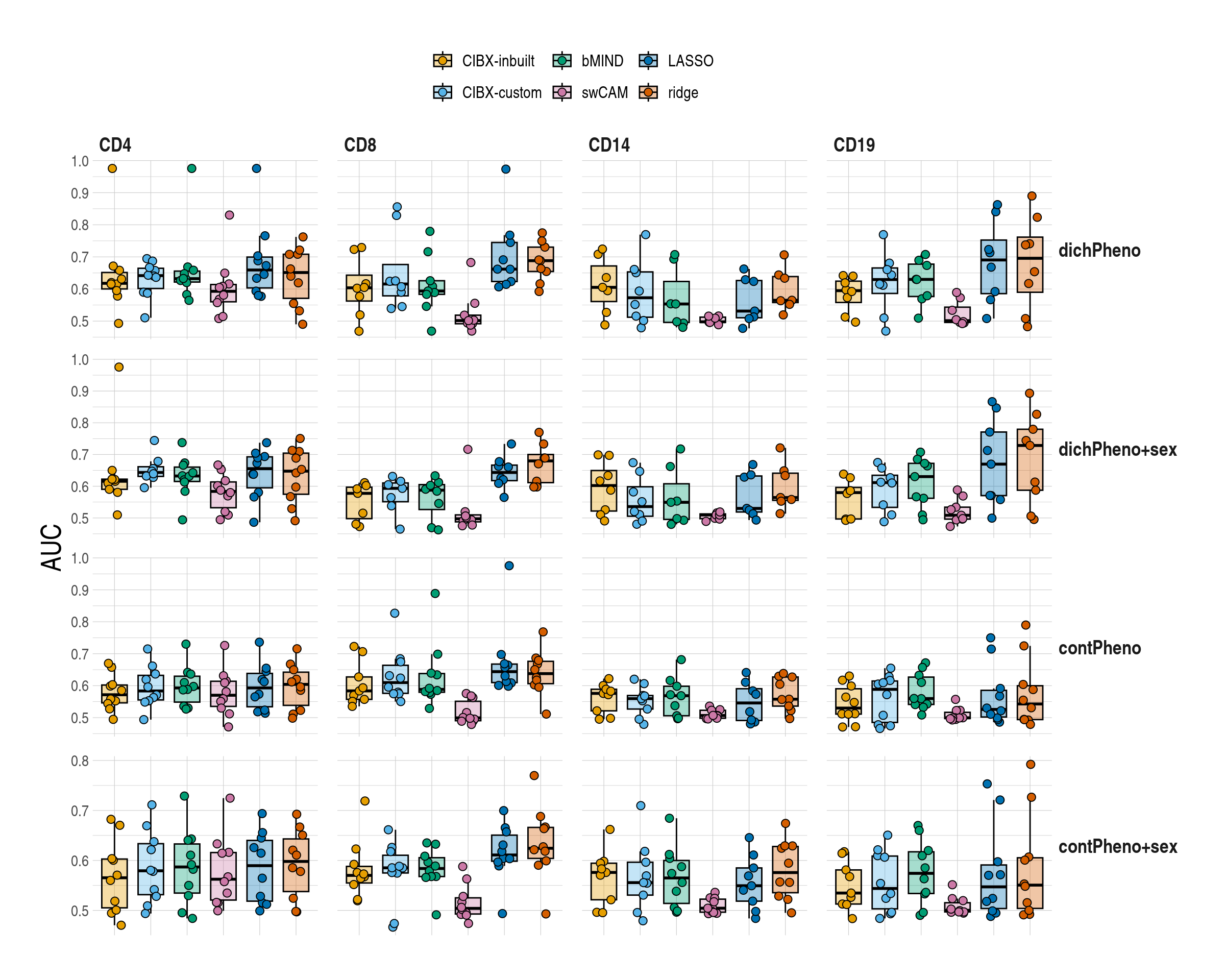

Code

mychktestonly_tbl <- copy(mychktestonly)
mychktestonly_tbl[, .N, by = c("scenarios", "celltype", "approach")]
             scenarios celltype approach  N
  1:   main.dcht.nocov      CD4  inbuilt 10
  2:   main.dcht.nocov      CD4   custom 10
  3:   main.dcht.nocov      CD4    bMIND 10
  4:   main.dcht.nocov      CD4    swCAM 10
  5:   main.dcht.nocov      CD4    LASSO 10
 ---                                       
188: common.cntn.covin     CD19   custom 10
189: common.cntn.covin     CD19    bMIND 10
190: common.cntn.covin     CD19    swCAM 10
191: common.cntn.covin     CD19    LASSO 10
192: common.cntn.covin     CD19    RIDGE 10

tbl_summary <- mychktestonly_tbl[, list(
  Q50 = median(auc, na.rm = TRUE) %>% round(., 2),
  Q25 = quantile(auc, probs = 0.25, na.rm = TRUE) %>% round(., 2),
  Q75 = quantile(auc, probs = 0.75, na.rm = TRUE) %>% round(., 2)
),
by = c("scenarios", "celltype", "approach")
][
  , V1 := paste0(Q50, " (", Q25, "-", Q75, ")")
]

tbl_summary[, pheno := gsub("^main\\.|^common\\.", "", scenarios)]
tbl_summary[, scenario := str_extract(scenarios, "main|common")]

tbl_res <- dcast(
  data = tbl_summary, pheno + celltype ~ scenario + approach,
  value.var = "V1"
)

setDF(tbl_res, rownames = paste0(tbl_res$pheno, tbl_res$celltype))

pheno.order <- CJ(c("dcht", "cntn"), c("nocov", "covin"), sorted = FALSE)[, paste(V1, V2, sep = ".")]

cols.order <- CJ(c("main", "common"), V2 = expr_order, sorted = FALSE)[, paste(V1, V2, sep = "_")]

rows.order <- CJ(pheno.order, sctorder, sorted = FALSE)[, paste0(pheno.order, sctorder)]

tbl_out <- tbl_res[rows.order, c("celltype", grep("main", cols.order, value = TRUE))]
names(tbl_out) <- gsub("main_|common_", "", names(tbl_out))

capin <- paste0(
  "Median AUC (Q25-Q75) across",
  ifelse(nrow(achk) != 0, "", uniqueN(mychktestonly$fakedPCs)),
  " simulated phentoypes per cell by apparoch. **Genes common across approaches per cell type**"
)


kbl(
  x = tbl_out, row.names = FALSE,
  caption = capin
) %>%
  kable_paper("striped", full_width = FALSE) %>%
  pack_rows("dichotomous pheno", 1, 4,
    label_row_css = "text-align: left;"
  ) %>%
  pack_rows("dichotomous pheno + sex", 5, 8) %>%
  pack_rows("continous pheno", 9, 12) %>%
  pack_rows("continous pheno + sex", 13, 16) %>%
  column_spec(column = 6:7, bold = T)

Median AUC (Q25-Q75) across simulated phentoypes per cell by apparoch. **Genes common across approaches per cell type**
celltype	inbuilt	custom	bMIND	swCAM	LASSO	RIDGE
dichotomous pheno
CD4	0.62 (0.6-0.65)	0.64 (0.6-0.66)	0.63 (0.62-0.66)	0.59 (0.56-0.61)	0.66 (0.6-0.7)	0.65 (0.57-0.71)
CD8	0.6 (0.56-0.64)	0.62 (0.58-0.68)	0.59 (0.58-0.63)	0.5 (0.49-0.52)	0.66 (0.62-0.74)	0.69 (0.65-0.73)
CD14	0.61 (0.56-0.67)	0.57 (0.51-0.65)	0.55 (0.5-0.62)	0.5 (0.5-0.51)	0.53 (0.51-0.63)	0.56 (0.56-0.64)
CD19	0.59 (0.56-0.62)	0.63 (0.59-0.67)	0.63 (0.58-0.68)	0.5 (0.5-0.54)	0.69 (0.59-0.75)	0.7 (0.59-0.76)
dichotomous pheno + sex
CD4	0.62 (0.59-0.62)	0.64 (0.63-0.66)	0.63 (0.61-0.66)	0.58 (0.53-0.61)	0.66 (0.59-0.69)	0.65 (0.57-0.7)
CD8	0.58 (0.5-0.6)	0.59 (0.55-0.61)	0.59 (0.53-0.61)	0.5 (0.49-0.51)	0.64 (0.62-0.67)	0.68 (0.61-0.7)
CD14	0.6 (0.52-0.65)	0.54 (0.51-0.6)	0.55 (0.5-0.61)	0.51 (0.5-0.51)	0.53 (0.52-0.63)	0.56 (0.56-0.64)
CD19	0.58 (0.5-0.6)	0.61 (0.53-0.63)	0.63 (0.56-0.67)	0.51 (0.5-0.53)	0.67 (0.57-0.77)	0.73 (0.59-0.78)
continous pheno
CD4	0.57 (0.55-0.6)	0.58 (0.56-0.63)	0.59 (0.55-0.63)	0.57 (0.54-0.61)	0.59 (0.53-0.64)	0.6 (0.54-0.64)
CD8	0.58 (0.56-0.63)	0.61 (0.58-0.66)	0.59 (0.58-0.64)	0.5 (0.49-0.55)	0.64 (0.61-0.67)	0.64 (0.61-0.68)
CD14	0.58 (0.52-0.59)	0.56 (0.53-0.57)	0.57 (0.51-0.6)	0.51 (0.5-0.52)	0.55 (0.49-0.59)	0.56 (0.54-0.63)
CD19	0.53 (0.51-0.59)	0.59 (0.48-0.61)	0.56 (0.54-0.63)	0.5 (0.5-0.52)	0.53 (0.5-0.59)	0.54 (0.49-0.6)
continous pheno + sex
CD4	0.57 (0.51-0.6)	0.58 (0.53-0.63)	0.59 (0.53-0.63)	0.56 (0.52-0.62)	0.59 (0.52-0.64)	0.6 (0.54-0.64)
CD8	0.57 (0.55-0.59)	0.59 (0.57-0.61)	0.58 (0.57-0.61)	0.5 (0.49-0.53)	0.61 (0.6-0.65)	0.62 (0.6-0.67)
CD14	0.58 (0.52-0.59)	0.56 (0.53-0.6)	0.56 (0.51-0.6)	0.5 (0.5-0.52)	0.55 (0.52-0.58)	0.58 (0.54-0.63)
CD19	0.53 (0.51-0.58)	0.54 (0.5-0.61)	0.57 (0.53-0.62)	0.5 (0.5-0.52)	0.55 (0.5-0.59)	0.55 (0.5-0.61)

2.14.2 Common gene sets

Code

achk1 <- mychktestonly[scenario == "common" & !is.na(auc), .N, by = c("pheno", "celltype", "approach")][N != 10, ]
achk1
            pheno celltype approach N
 1:     dichPheno      CD8  inbuilt 8
 2:     dichPheno      CD8   custom 8
 3:     dichPheno      CD8    bMIND 8
 4:     dichPheno      CD8    swCAM 8
 5:     dichPheno      CD8    LASSO 8
 6:     dichPheno      CD8    RIDGE 8
 7:     dichPheno     CD14  inbuilt 7
 8:     dichPheno     CD14   custom 7
 9:     dichPheno     CD14    bMIND 7
10:     dichPheno     CD14    swCAM 7
11:     dichPheno     CD14    LASSO 7
12:     dichPheno     CD14    RIDGE 7
13:     dichPheno     CD19  inbuilt 7
14:     dichPheno     CD19   custom 7
15:     dichPheno     CD19    bMIND 7
16:     dichPheno     CD19    swCAM 7
17:     dichPheno     CD19    LASSO 7
18:     dichPheno     CD19    RIDGE 7
19: dichPheno+sex      CD4  inbuilt 9
20: dichPheno+sex      CD4   custom 9
21: dichPheno+sex      CD4    bMIND 9
22: dichPheno+sex      CD4    swCAM 9
23: dichPheno+sex      CD4    LASSO 9
24: dichPheno+sex      CD4    RIDGE 9
25: dichPheno+sex      CD8  inbuilt 7
26: dichPheno+sex      CD8   custom 7
27: dichPheno+sex      CD8    bMIND 7
28: dichPheno+sex      CD8    swCAM 7
29: dichPheno+sex      CD8    LASSO 7
30: dichPheno+sex      CD8    RIDGE 7
31: dichPheno+sex     CD14  inbuilt 7
32: dichPheno+sex     CD14   custom 7
33: dichPheno+sex     CD14    bMIND 7
34: dichPheno+sex     CD14    swCAM 7
35: dichPheno+sex     CD14    LASSO 7
36: dichPheno+sex     CD14    RIDGE 7
37: dichPheno+sex     CD19  inbuilt 8
38: dichPheno+sex     CD19   custom 8
39: dichPheno+sex     CD19    bMIND 8
40: dichPheno+sex     CD19    swCAM 8
41: dichPheno+sex     CD19    LASSO 8
42: dichPheno+sex     CD19    RIDGE 8
43:     contPheno      CD8  inbuilt 9
44:     contPheno      CD8   custom 9
45:     contPheno      CD8    bMIND 9
46:     contPheno      CD8    swCAM 9
47:     contPheno      CD8    LASSO 9
48:     contPheno      CD8    RIDGE 9
49:     contPheno     CD14  inbuilt 9
50:     contPheno     CD14   custom 9
51:     contPheno     CD14    bMIND 9
52:     contPheno     CD14    swCAM 9
53:     contPheno     CD14    LASSO 9
54:     contPheno     CD14    RIDGE 9
55:     contPheno     CD19  inbuilt 9
56:     contPheno     CD19   custom 9
57:     contPheno     CD19    bMIND 9
58:     contPheno     CD19    swCAM 9
59:     contPheno     CD19    LASSO 9
60:     contPheno     CD19    RIDGE 9
61: contPheno+sex     CD14  inbuilt 9
62: contPheno+sex     CD14   custom 9
63: contPheno+sex     CD14    bMIND 9
64: contPheno+sex     CD14    swCAM 9
65: contPheno+sex     CD14    LASSO 9
66: contPheno+sex     CD14    RIDGE 9
67: contPheno+sex     CD19  inbuilt 9
68: contPheno+sex     CD19   custom 9
69: contPheno+sex     CD19    bMIND 9
70: contPheno+sex     CD19    swCAM 9
71: contPheno+sex     CD19    LASSO 9
72: contPheno+sex     CD19    RIDGE 9
            pheno celltype approach N

ggboxplot(
  data = mychktestonly[scenario == "common", ],
  x = "approach", y = "auc", ylab = "AUC",
  palette = appro.cols,
  alpha = 0.35, fill = "approach",
  add = c("jitter"),
  add.params = list(shape = 21, size = 2.5, alpha = 1)
) +
  scale_fill_manual(labels = appro_lab, values = appro.cols) +
  facet_grid(pheno ~ celltype, scales = "free") +
  labs(fill = NULL) +
  used_ggthemes(
    axis.text.x = element_blank(),
    legend.position = "top",
    strip.text.y.right = element_text(angle = 0),
    legend.text = element_text(size = rel(1))
  ) +
  rremove("xlab")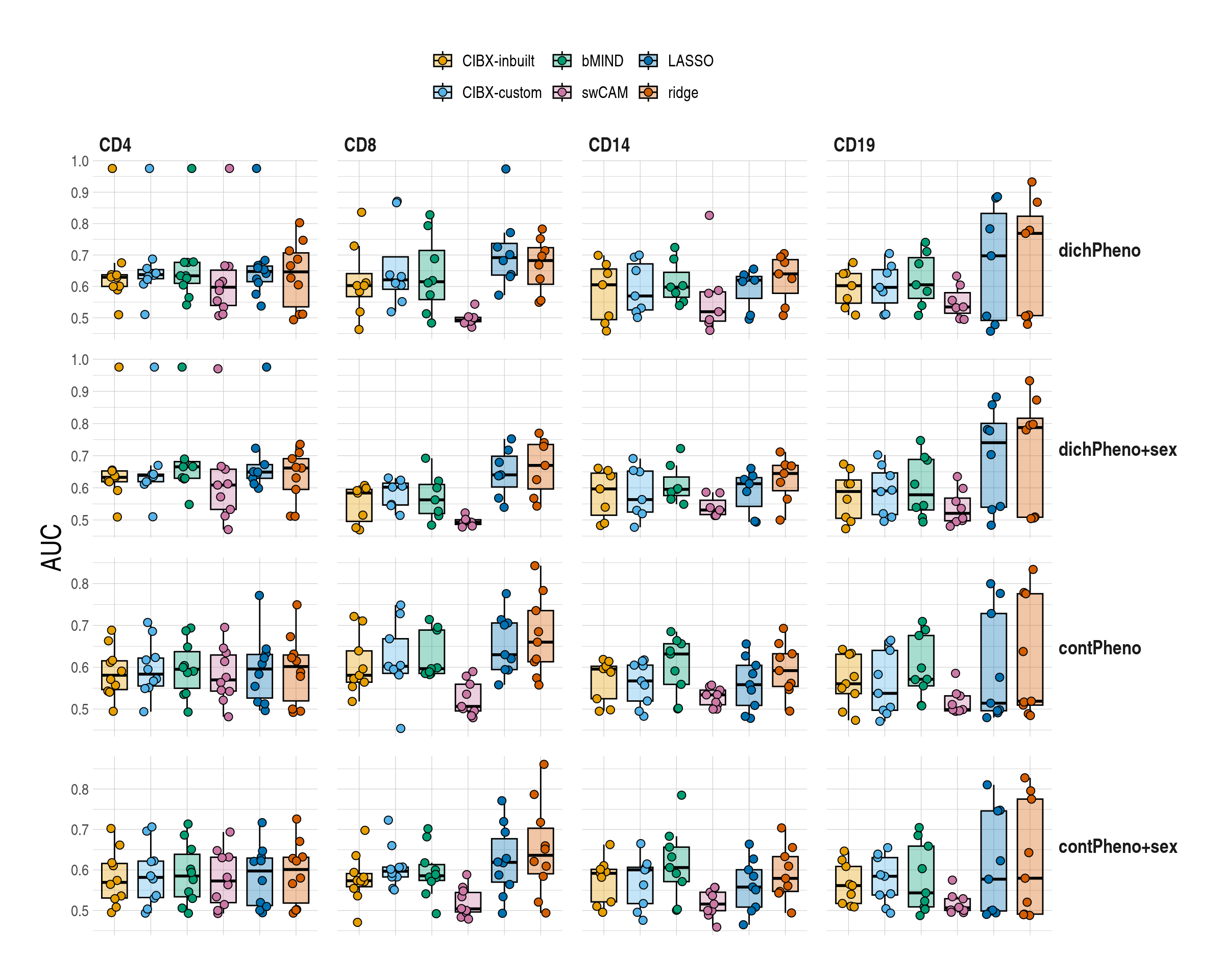

Differential gene expression (DGE) recovery. **Genes common across approaches were used**. No. common genes are 3837 for CD4, 6274 for CD8, 5185 for CD14, and 2689 for CD19 Area under curve (AUC) distributions by cell type (columns) and approach for each scenario (rows). **dichPheno: simulated dichotomous phenotype; dichPheno+sex: simulated dichotomous phenotype and sex; contPheno: continous phenotype; contPheno+sex: continous phenotype and sex**. Each point is a simulated phenotype, and ten phenotypes were simulated. For each simulated phenotype, the receiver operating characteristic curve and AUC were estimated by FDR fixed at 0.05 in the observed data and varied FDRs from 0 to 1 by 0.05 in the imputed data. Box plots showed the AUC distributions, with horizontal lines from the bottom to the top for 25 %, 50 % and 75 % quantiles, respectively. inbuilt: CIBERSORTx with the inbuilt signature matrix; custom: CIBERSORTx with a custom signature matrix; bMIND: bMIND with flow fractions; swCAM: swCAM with flow fractions; LASSO/RIDGE: regularised multi-response Gaussian models. Noted AUC was not calculated for some simulated phenotypes because all associations were true negative, and none were false negative. Scenario-celltype-approach with no. AUCs \(<\) 10 are listed in the code chunk.

Code

tbl_out <- tbl_res[rows.order, c("celltype", grep("common", cols.order, value = TRUE))]
names(tbl_out) <- gsub("main_|common_", "", names(tbl_out))

capin <- paste0(
  "Median AUC (Q25-Q75) across",
  ifelse(nrow(achk1) != 0, "", uniqueN(mychktestonly$fakedPCs)),
  " simulated phentoypes per cell by apparoch. **Genes common across approaches per cell type**"
)

kbl(
  x = tbl_out, row.names = FALSE,
  caption = capin
) %>%
  kable_paper("striped", full_width = FALSE) %>%
  column_spec(column = 6:7, bold = TRUE) %>%
  pack_rows("dichotomous pheno", 1, 4,
    label_row_css = "text-align: left;"
  ) %>%
  pack_rows("dichotomous pheno + sex", 5, 8) %>%
  pack_rows("continous pheno", 9, 12) %>%
  pack_rows("continous pheno + sex", 13, 16)

Median AUC (Q25-Q75) across simulated phentoypes per cell by apparoch. **Genes common across approaches per cell type**
celltype	inbuilt	custom	bMIND	swCAM	LASSO	RIDGE
dichotomous pheno
CD4	0.63 (0.6-0.64)	0.64 (0.62-0.65)	0.63 (0.61-0.68)	0.6 (0.54-0.65)	0.65 (0.62-0.66)	0.65 (0.54-0.71)
CD8	0.6 (0.57-0.64)	0.62 (0.59-0.69)	0.61 (0.56-0.71)	0.49 (0.49-0.5)	0.69 (0.64-0.74)	0.68 (0.61-0.72)
CD14	0.61 (0.49-0.66)	0.57 (0.53-0.67)	0.6 (0.57-0.64)	0.52 (0.49-0.58)	0.62 (0.56-0.63)	0.64 (0.58-0.69)
CD19	0.6 (0.55-0.64)	0.6 (0.55-0.65)	0.61 (0.56-0.69)	0.53 (0.51-0.58)	0.7 (0.49-0.83)	0.77 (0.51-0.82)
dichotomous pheno + sex
CD4	0.63 (0.62-0.65)	0.64 (0.62-0.64)	0.67 (0.63-0.68)	0.61 (0.53-0.66)	0.65 (0.63-0.67)	0.66 (0.59-0.69)
CD8	0.58 (0.5-0.6)	0.6 (0.55-0.61)	0.56 (0.52-0.61)	0.49 (0.49-0.5)	0.64 (0.6-0.7)	0.67 (0.6-0.73)
CD14	0.6 (0.51-0.65)	0.56 (0.52-0.65)	0.6 (0.58-0.63)	0.53 (0.52-0.56)	0.61 (0.54-0.63)	0.64 (0.59-0.67)
CD19	0.59 (0.51-0.62)	0.59 (0.52-0.65)	0.58 (0.53-0.69)	0.52 (0.5-0.57)	0.74 (0.54-0.8)	0.79 (0.51-0.82)
continous pheno
CD4	0.58 (0.55-0.62)	0.58 (0.56-0.62)	0.6 (0.55-0.64)	0.57 (0.54-0.63)	0.6 (0.53-0.63)	0.6 (0.52-0.63)
CD8	0.58 (0.56-0.64)	0.6 (0.59-0.67)	0.6 (0.59-0.69)	0.51 (0.5-0.56)	0.63 (0.59-0.71)	0.66 (0.61-0.74)
CD14	0.6 (0.52-0.6)	0.57 (0.52-0.61)	0.63 (0.56-0.66)	0.53 (0.51-0.55)	0.56 (0.51-0.6)	0.59 (0.55-0.63)
CD19	0.56 (0.54-0.63)	0.54 (0.5-0.64)	0.57 (0.56-0.68)	0.5 (0.5-0.53)	0.51 (0.5-0.73)	0.52 (0.51-0.78)
continous pheno + sex
CD4	0.57 (0.53-0.62)	0.58 (0.53-0.62)	0.59 (0.53-0.64)	0.57 (0.52-0.63)	0.6 (0.51-0.63)	0.6 (0.52-0.63)
CD8	0.57 (0.56-0.59)	0.6 (0.58-0.61)	0.59 (0.57-0.61)	0.5 (0.5-0.54)	0.62 (0.57-0.68)	0.64 (0.59-0.7)
CD14	0.59 (0.52-0.6)	0.6 (0.52-0.61)	0.61 (0.57-0.66)	0.52 (0.5-0.55)	0.56 (0.51-0.6)	0.58 (0.55-0.63)
CD19	0.56 (0.52-0.61)	0.58 (0.54-0.63)	0.54 (0.51-0.66)	0.51 (0.5-0.53)	0.58 (0.5-0.75)	0.58 (0.49-0.77)

2.15 AUCs in pseudo datasets

testing samples + varying gene sets

Code

simres_pltlist$main$sce2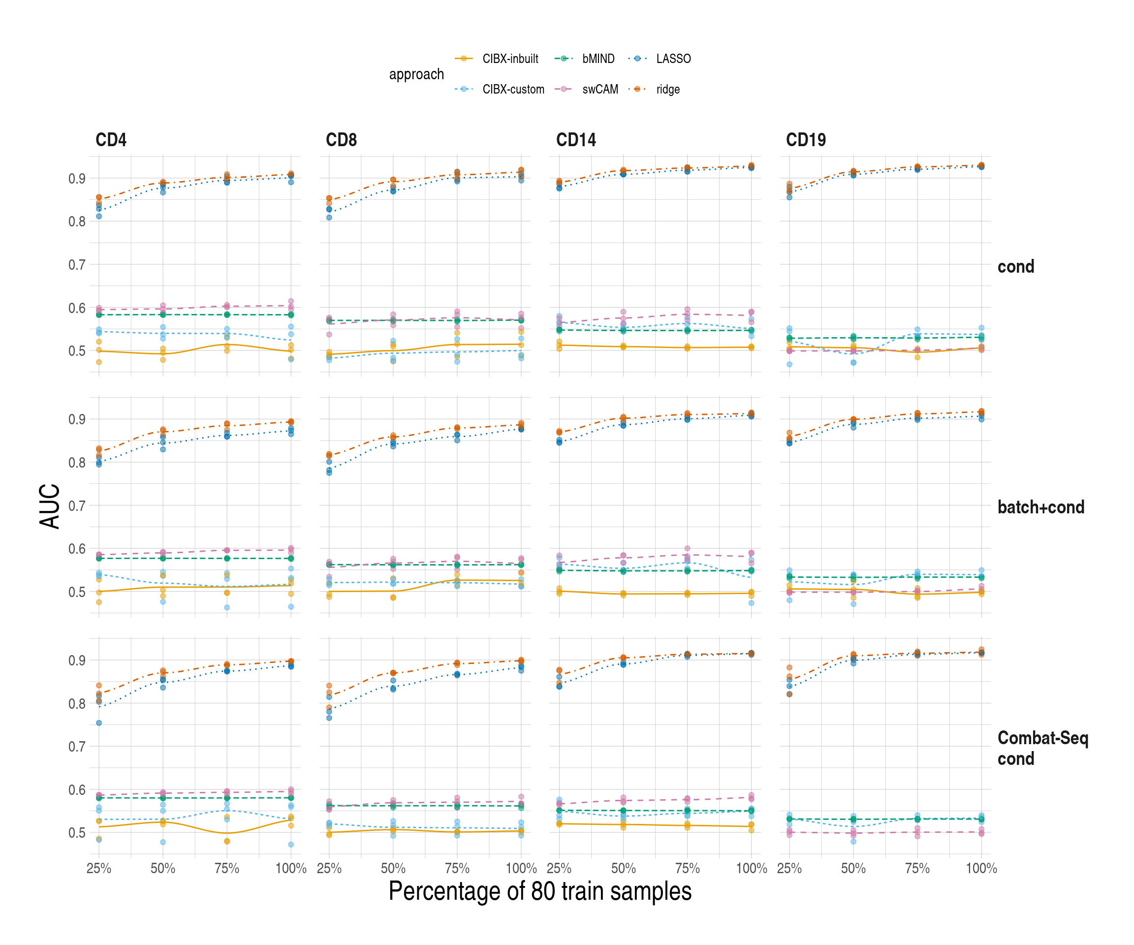

2.16 AUCs in pseudo datasets

testing samples + common gene set

Code

simres_pltlist$common$sce2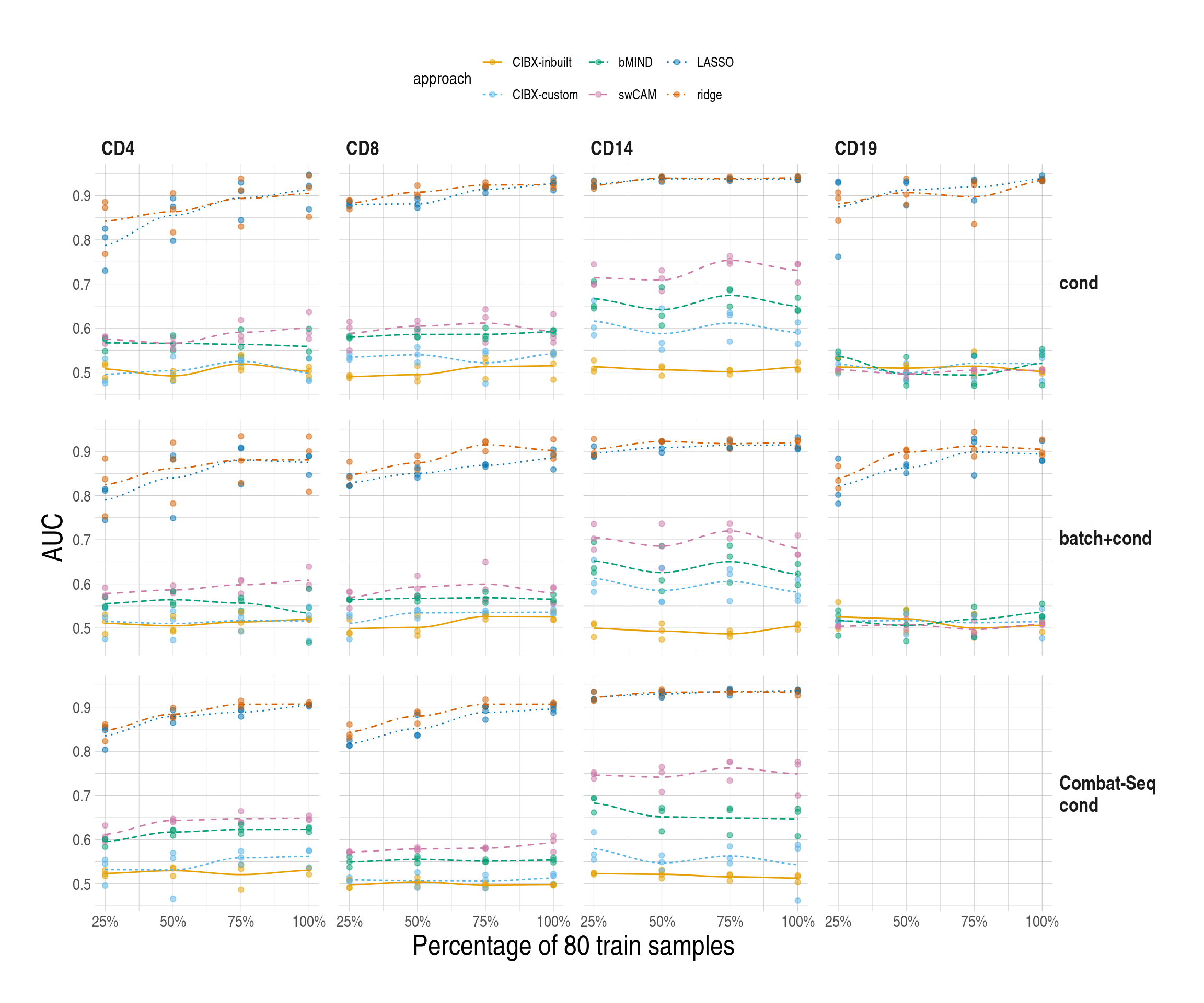

Session info

R version 4.3.3 (2024-02-29)
Platform: x86_64-pc-linux-gnu (64-bit)
Running under: Rocky Linux 8.10 (Green Obsidian)

Matrix products: default
BLAS/LAPACK: /usr/lib64/libopenblas-r0.3.15.so;  LAPACK version 3.9.0

locale:
 [1] LC_CTYPE=en_GB.UTF-8       LC_NUMERIC=C              
 [3] LC_TIME=en_GB.UTF-8        LC_COLLATE=en_GB.UTF-8    
 [5] LC_MONETARY=en_GB.UTF-8    LC_MESSAGES=en_GB.UTF-8   
 [7] LC_PAPER=en_GB.UTF-8       LC_NAME=C                 
 [9] LC_ADDRESS=C               LC_TELEPHONE=C            
[11] LC_MEASUREMENT=en_GB.UTF-8 LC_IDENTIFICATION=C       

time zone: GB
tzcode source: system (glibc)

attached base packages:
[1] grid      parallel  stats     graphics  grDevices datasets  utils    
[8] methods   base     

other attached packages:
 [1] circlize_0.4.16       cowplot_1.1.1         pROC_1.18.4          
 [4] kableExtra_1.3.4.9000 cols4all_0.7-1        ggpubr_0.6.0         
 [7] edgeR_3.42.4          limma_3.56.2          gridExtra_2.3        
[10] ggrepel_0.9.3         RColorBrewer_1.1-3    ggplot2_3.5.1        
[13] ComplexHeatmap_2.18.0 styler_1.10.2         knitr_1.44           
[16] stringr_1.5.0         magrittr_2.0.3        data.table_1.14.8    
[19] doParallel_1.0.17     iterators_1.0.14      foreach_1.5.2        

loaded via a namespace (and not attached):
  [1] rstudioapi_0.15.0       jsonlite_1.8.7          shape_1.4.6            
  [4] farver_2.1.1            rmarkdown_2.25          GlobalOptions_0.1.2    
  [7] vctrs_0.6.5             rstatix_0.7.2           webshot_0.5.5          
 [10] htmltools_0.5.6.1       polynom_1.4-1           curl_5.1.0             
 [13] broom_1.0.5             htmlwidgets_1.6.2       plyr_1.8.9             
 [16] mime_0.12               lifecycle_1.0.4         pkgconfig_2.0.3        
 [19] Matrix_1.6-5            R6_2.5.1                fastmap_1.1.1          
 [22] shiny_1.7.5             clue_0.3-65             digest_0.6.33          
 [25] colorspace_2.1-0        S4Vectors_0.38.2        rprojroot_2.0.3        
 [28] labeling_0.4.3          spacesXYZ_1.3-0         fansi_1.0.5            
 [31] httr_1.4.7              abind_1.4-5             mgcv_1.9-1             
 [34] compiler_4.3.3          here_1.0.1              fontquiver_0.2.1       
 [37] withr_2.5.1             backports_1.4.1         carData_3.0-5          
 [40] highr_0.10              Rttf2pt1_1.3.12         R.utils_2.12.2         
 [43] ggsignif_0.6.4          MASS_7.3-60.0.1         rjson_0.2.21           
 [46] ggpp_0.5.8-1            ggsci_3.0.0             gfonts_0.2.0           
 [49] tools_4.3.3             zip_2.3.0               httpuv_1.6.11          
 [52] extrafontdb_1.0         R.oo_1.25.0             glue_1.7.0             
 [55] nlme_3.1-164            R.cache_0.16.0          promises_1.2.1         
 [58] cluster_2.1.6           generics_0.1.3          gtable_0.3.4           
 [61] R.methodsS3_1.8.2       tidyr_1.3.0             xml2_1.3.5             
 [64] car_3.1-2               utf8_1.2.3              BiocGenerics_0.46.0    
 [67] pillar_1.9.0            later_1.3.1             splines_4.3.3          
 [70] dplyr_1.1.4             lattice_0.22-5          renv_1.0.10            
 [73] tidyselect_1.2.0        fontLiberation_0.1.0    locfit_1.5-9.8         
 [76] fontBitstreamVera_0.1.1 IRanges_2.34.1          svglite_2.1.2          
 [79] crul_1.4.0              stats4_4.3.3            xfun_0.40              
 [82] matrixStats_1.0.0       pheatmap_1.0.12         stringi_1.7.12         
 [85] yaml_2.3.7              evaluate_0.22           codetools_0.2-19       
 [88] httpcode_0.3.0          extrafont_0.19          gdtools_0.3.3          
 [91] tibble_3.2.1            BiocManager_1.30.22     cli_3.6.2              
 [94] xtable_1.8-4            systemfonts_1.0.5       munsell_0.5.0          
 [97] Rcpp_1.0.11             png_0.1-8               ellipsis_0.3.2         
[100] viridisLite_0.4.2       hrbrthemes_0.8.0        scales_1.3.0           
[103] openxlsx_4.2.5.2        purrr_1.0.2             crayon_1.5.2           
[106] GetoptLong_1.0.5        rlang_1.1.3             rvest_1.0.3